Mapping migration

Introduction to vector data operations

Learning Goals:

Combine different types of vector data with spatial joins
Create a chloropleth plot

The Veery thrush (Catharus fuscescens) migrates each year between nesting sites in the U.S. and Canada, and South America. Veeries are small birds, and encountering a hurricane during their migration would be disasterous. However, Ornithologist Christopher Hechscher has found in tracking their migration that their breeding patterns and migration timing can predicting the severity of hurricane season as accurately as meterological models (Heckscher 2018)!

Veery in Central Park by the Ramble Stone Arch. Source: Wikimedia

You can read more about the Veery migration and how climate change may be impacting these birds in this article from the Audobon Society, or in Heckscher’s open access report.

Check out our demo video!

DEMO: Migration Part 1 (EDA) by Earth Lab

DEMO: Migration Part 2 (EDA) by Earth Lab

DEMO: Migration Part 3 (EDA) by Earth Lab

Reflect and Respond: What can we learn from migration patterns?

Reflect on what you know about migration. You could consider:

What are some reasons that animals migrate?
How might climate change affect animal migrations?
Do you notice any animal migrations in your area?

id = 'eda'
species_name = 'Veery Thrush'
species_lookup = 'catharus fuscescens'
sample_filename = 'migration-foundations-data'
download_filename = 'gbif_veery'
plot_filename = 'veery_migration'
plot_height = 800

STEP 1: Set up your reproducible workflow

Import Python libraries

Try It: Import packages

In the imports cell, we’ve included some packages that you will need. Add imports for packages that will help you:

Work with tabular data
Work with geospatial vector data

import os
import pathlib

See our solution!

import os
import pathlib

import geopandas as gpd
import pandas as pd

Create a folder for your data

For this challenge, you will need to save some data to the computer you’re working on. We suggest saving to somewhere in your home folder (e.g. /home/username), rather than to your GitHub repository, since data files can easily become too large for GitHub.

Warning

The home directory is different for every user! Your home directory probably won’t exist on someone else’s computer. Make sure to use code like pathlib.Path.home() to compute the home directory on the computer the code is running on. This is key to writing reproducible and interoperable code.

Try It: Create a project folder

The code below will help you get started with making a project directory

Replace 'your-project-directory-name-here' and 'your-gbif-data-directory-name-here' with descriptive names
Run the cell
(OPTIONAL) Check in the terminal that you created the directory using the command ls ~/earth-analytics/data

# Create data directory in the home folder
data_dir = os.path.join(
    # Home directory
    pathlib.Path.home(),
    # Earth analytics data directory
    'earth-analytics',
    'data',
    # Project directory
    'your-project-directory-name-here',
)
os.makedirs(data_dir, exist_ok=True)

See our solution!

# Create data directory in the home folder
data_dir = os.path.join(
    pathlib.Path.home(),
    'earth-analytics',
    'data',
    'migration',
)
os.makedirs(data_dir, exist_ok=True)

STEP 2: Define your study area – the ecoregions of North America

Track observations of Veery Thrush across different ecoregions! You should be able to see changes in the number of observations in each ecoregion throughout the year.

The ecoregion data will be available as a shapefile. Learn more about shapefiles and vector data in this Introduction to Spatial Vector Data File Formats in Open Source Python

Download and save ecoregion boundaries

The ecoregion boundaries take some time to download – they come in at about 150MB. To use your time most efficiently, we recommend caching the ecoregions data on the machine you’re working on so that you only have to download once. To do that, we’ll also introduce the concept of conditionals, or code that adjusts what it does based on the situation.

Read more about conditionals in this Intro Conditional Statements in Python

Try It: Get ecoregions boundaries

Find the URL for for the ecoregion boundary Shapefile. You can get ecoregion boundaries from Google..
Replace your/url/here with the URL you found, making sure to format it so it is easily readable. Also, replace ecoregions_dirname and ecoregions_filename with descriptive and machine-readable names for your project’s file structure.
Change all the variable names to descriptive variable names, making sure to correctly reference variables you created before.
Run the cell to download and save the data.

# Set up the ecoregion boundary URL
url = "your/url/here"

# Set up a path to save the data on your machine
the_dir = os.path.join(project_data_dir, 'ecoregions_dirname')
# Make the ecoregions directory

# Join ecoregions shapefile path
a_path = os.path.join(the_dir, 'ecoregions_filename.shp')

# Only download once
if not os.path.exists(a_path):
    my_gdf = gpd.read_file(your_url_here)
    my_gdf.to_file(your_path_here)

See our solution!

# Set up the ecoregion boundary URL
ecoregions_url = (
    "https://storage.googleapis.com/teow2016/Ecoregions2017.zip")

# Set up a path to save the data on your machine
ecoregions_dir = os.path.join(data_dir, 'wwf_ecoregions')
os.makedirs(ecoregions_dir, exist_ok=True)
ecoregions_path = os.path.join(ecoregions_dir, 'wwf_ecoregions.shp')

# Only download once
if not os.path.exists(ecoregions_path):
    ecoregions_gdf = gpd.read_file(ecoregions_url)
    ecoregions_gdf.to_file(ecoregions_path)

ERROR 1: PROJ: proj_create_from_database: Open of /usr/share/miniconda/envs/learning-portal/share/proj failed

Let’s check that that worked! To do so we’ll use a bash command called find to look for all the files in your project directory with the .shp extension:

%%bash
find ~/earth-analytics/data/migration -name '*.shp'

/home/runner/earth-analytics/data/migration/wwf_ecoregions/wwf_ecoregions.shp

Tip

You can also run bash commands in the terminal!

Learn more about bash in this Introduction to Bash

Load the ecoregions into Python

Try It: Load ecoregions into Python

Download and save ecoregion boundaries from the EPA:

Replace a_path with the path your created for your ecoregions file.
(optional) Consider renaming and selecting columns to make your GeoDataFrame easier to work with. Many of the same methods you learned for pandas DataFrames are the same for GeoDataFrames! NOTE: Make sure to keep the 'SHAPE_AREA' column around – we will need that later!
Make a quick plot with .plot() to make sure the download worked.
Run the cell to load the data into Python

# Open up the ecoregions boundaries
gdf = gpd.read_file(a_path)

# Name the index so it will match the other data later on
gdf.index.name = 'ecoregion'

# Plot the ecoregions to check download

See our solution!

# Open up the ecoregions boundaries
ecoregions_gdf = (
    gpd.read_file(ecoregions_path)
    .rename(columns={
        'ECO_NAME': 'name',
        'SHAPE_AREA': 'area'})
    [['name', 'area', 'geometry']]
)

# We'll name the index so it will match the other data
ecoregions_gdf.index.name = 'ecoregion'

# Plot the ecoregions to check download
ecoregions_gdf.plot(edgecolor='black', color='skyblue')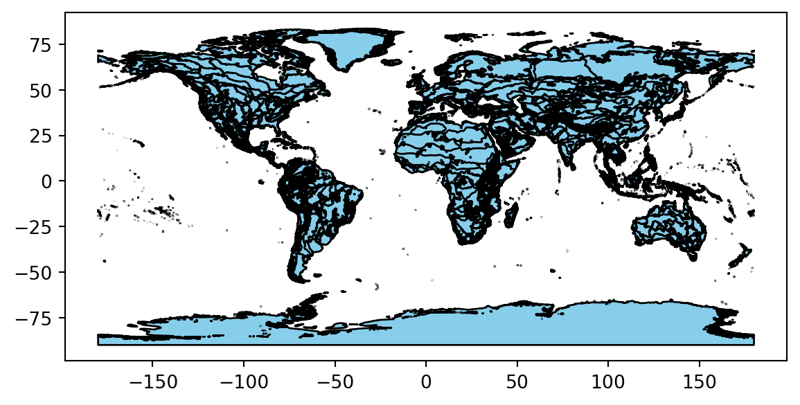

STEP 3: Download species observation data

For this challenge, you will use a database called the Global Biodiversity Information Facility (GBIF). GBIF is compiled from species observation data all over the world, and includes everything from museum specimens to photos taken by citizen scientists in their backyards. We’ve compiled some sample data in the same format that you will get from GBIF.

Download sample data

Try It: Import GBIF Data

Define the gbif_url to be this sample data URL { params.sample_url }
Using the ecoregions code, modify the code cell below so that the download only runs once, as with the ecoregion data.
Run the cell

# Load the GBIF data
gbif_df = pd.read_csv(
    gbif_url, 
    delimiter='\t',
    index_col='gbifID',
    usecols=['gbifID', 'decimalLatitude', 'decimalLongitude', 'month'])
gbif_df.head()

See our solution!

# Define the sample data URL
gbif_url = (
    "https://github.com/cu-esiil-edu/esiil-learning-portal/releases/download"
    f"/data-release/{ sample_filename }.zip")
    
# Set up a path to save the data on your machine
gbif_filename = download_filename
gbif_dir = os.path.join(data_dir, gbif_filename)
os.makedirs(gbif_dir, exist_ok=True)
gbif_path = os.path.join(gbif_dir, f"{ gbif_filename }.zip")

# Only download once
if not os.path.exists(gbif_path):
    # Load the GBIF data
    gbif_df = pd.read_csv(
        gbif_url, 
        delimiter='\t',
        index_col='gbifID',
        usecols=['gbifID', 'decimalLatitude', 'decimalLongitude', 'month'])
    # Save the GBIF data
    gbif_df.to_csv(gbif_path, index=False)

gbif_df = pd.read_csv(gbif_path)
gbif_df.head()

	decimalLatitude	decimalLongitude	month
0	40.771550	-73.97248	9
1	42.588123	-85.44625	5
2	43.703064	-72.30729	5
3	48.174270	-77.73126	7
4	42.544277	-72.44836	5

Convert the GBIF data to a GeoDataFrame

To plot the GBIF data, we need to convert it to a GeoDataFrame first. This will make some special geospatial operations from geopandas available, such as spatial joins and plotting.

Try It: Convert `DataFrame` to `GeoDataFrame`

Replace your_dataframe with the name of the DataFrame you just got from GBIF
Replace longitude_column_name and latitude_column_name with column names from your `DataFrame
Run the code to get a GeoDataFrame of the GBIF data.

gbif_gdf = (
    gpd.GeoDataFrame(
        your_dataframe, 
        geometry=gpd.points_from_xy(
            your_dataframe.longitude_column_name, 
            your_dataframe.latitude_column_name), 
        crs="EPSG:4326")
    # Select the desired columns
    [[]]
)
gbif_gdf

See our solution!

gbif_gdf = (
    gpd.GeoDataFrame(
        gbif_df, 
        geometry=gpd.points_from_xy(
            gbif_df.decimalLongitude, 
            gbif_df.decimalLatitude), 
        crs="EPSG:4326")
    # Select the desired columns
    [['month', 'geometry']]
)
gbif_gdf

	month	geometry
0	9	POINT (-73.97248 40.77155)
1	5	POINT (-85.44625 42.58812)
2	5	POINT (-72.30729 43.70306)
3	7	POINT (-77.73126 48.17427)
4	5	POINT (-72.44836 42.54428)
...	...	...
162770	5	POINT (-78.75946 45.0954)
162771	7	POINT (-88.02332 48.99255)
162772	5	POINT (-72.79677 43.46352)
162773	6	POINT (-81.32435 46.04416)
162774	5	POINT (-73.82481 40.61684)

162775 rows × 2 columns

STEP 4: Count the number of observations in each ecosystem, during each month of 2023

Much of the data in GBIF is crowd-sourced. As a result, we need not just the number of observations in each ecosystem each month – we need to normalize by some measure of sampling effort. After all, we wouldn’t expect the same number of observations at the North Pole as we would in a National Park, even if there were the same number organisms. In this case, we’re normalizing using the average number of observations for each ecosystem and each month. This should help control for the number of active observers in each location and time of year.

Identify the ecoregion for each observation

You can combine the ecoregions and the observations spatially using a method called .sjoin(), which stands for spatial join.

Check out the geopandas documentation on spatial joins to help you figure this one out. You can also ask your favorite LLM (Large-Language Model, like ChatGPT)

Try It: Perform a spatial join

Identify the correct values for the how= and predicate= parameters of the spatial join.
Select only the columns you will need for your plot.
Run the code.

gbif_ecoregion_gdf = (
    ecoregions_gdf
    # Match the CRS of the GBIF data and the ecoregions
    .to_crs(gbif_gdf.crs)
    # Find ecoregion for each observation
    .sjoin(
        gbif_gdf,
        how='', 
        predicate='')
    # Select the required columns
    
)
gbif_ecoregion_gdf

See our solution!

gbif_ecoregion_gdf = (
    ecoregions_gdf
    # Match the CRS of the GBIF data and the ecoregions
    .to_crs(gbif_gdf.crs)
    # Find ecoregion for each observation
    .sjoin(
        gbif_gdf,
        how='inner', 
        predicate='contains')
    # Select the required columns
    [['month', 'name']]
)
gbif_ecoregion_gdf

	month	name
ecoregion
12	5	Alberta-British Columbia foothills forests
12	5	Alberta-British Columbia foothills forests
12	6	Alberta-British Columbia foothills forests
12	7	Alberta-British Columbia foothills forests
12	6	Alberta-British Columbia foothills forests
...	...	...
839	10	North Atlantic moist mixed forests
839	9	North Atlantic moist mixed forests
839	9	North Atlantic moist mixed forests
839	9	North Atlantic moist mixed forests
839	9	North Atlantic moist mixed forests

159537 rows × 2 columns

Count the observations in each ecoregion each month

Try It: Group observations by ecoregion

Replace columns_to_group_by with a list of columns. Keep in mind that you will end up with one row for each group – you want to count the observations in each ecoregion by month.
Select only month/ecosystem combinations that have more than one occurrence recorded, since a single occurrence could be an error.
Use the .groupby() and .mean() methods to compute the mean occurrences by ecoregion and by month.
Run the code – it will normalize the number of occurrences by month and ecoretion.

occurrence_df = (
    gbif_ecoregion_gdf
    # For each ecoregion, for each month...
    .groupby(columns_to_group_by)
    # ...count the number of occurrences
    .agg(occurrences=('name', 'count'))
)

# Get rid of rare observations (possible misidentification?)
occurrence_df = occurrence_df[...]

# Take the mean by ecoregion
mean_occurrences_by_ecoregion = (
    occurrence_df
    ...
)
# Take the mean by month
mean_occurrences_by_month = (
    occurrence_df
    ...
)

See our solution!

occurrence_df = (
    gbif_ecoregion_gdf
    # For each ecoregion, for each month...
    .groupby(['ecoregion', 'month'])
    # ...count the number of occurrences
    .agg(occurrences=('name', 'count'))
)

# Get rid of rare observation noise (possible misidentification?)
occurrence_df = occurrence_df[occurrence_df.occurrences>1]

# Take the mean by ecoregion
mean_occurrences_by_ecoregion = (
    occurrence_df
    .groupby(['ecoregion'])
    .mean()
)
# Take the mean by month
mean_occurrences_by_month = (
    occurrence_df
    .groupby(['month'])
    .mean()
)

Normalize the observations

Try It: Normalize

Divide occurrences by the mean occurrences by month AND the mean occurrences by ecoregion

# Normalize by space and time for sampling effort
occurrence_df['norm_occurrences'] = (
    occurrence_df
    ...
)
occurrence_df

See our solution!

occurrence_df['norm_occurrences'] = (
    occurrence_df
    / mean_occurrences_by_ecoregion
    / mean_occurrences_by_month
)
occurrence_df

		occurrences	norm_occurrences
ecoregion	month
12	5	2	0.000828
	6	2	0.000960
	7	2	0.001746
16	4	2	0.000010
16	5	2980	0.001732
...	...	...	...
833	7	293	0.002173
	8	40	0.001030
	9	11	0.000179
839	9	25	0.005989
839	10	7	0.013328

308 rows × 2 columns

STEP 5: Plot the Veery Thrush observations by month

First thing first – let’s load your stored variables and import libraries.

%store -r ecoregions_gdf occurrence_df

Try It: Import packages

In the imports cell, we’ve included some packages that you will need. Add imports for packages that will help you:

Make interactive maps with vector data

# Get month names
import calendar

# Libraries for Dynamic mapping
import cartopy.crs as ccrs
import panel as pn

See our solution!

# Get month names
import calendar

# Libraries for Dynamic mapping
import cartopy.crs as ccrs
import hvplot.pandas
import panel as pn

Create a simplified `GeoDataFrame` for plotting

Plotting larger files can be time consuming. The code below will streamline plotting with hvplot by simplifying the geometry, projecting it to a Mercator projection that is compatible with geoviews, and cropping off areas in the Arctic.

Try It: Simplify ecoregion data

Download and save ecoregion boundaries from the EPA:

Simplify the ecoregions with .simplify(.05), and save it back to the geometry column.
Change the Coordinate Reference System (CRS) to Mercator with .to_crs(ccrs.Mercator())
Use the plotting code that is already in the cell to check that the plotting runs quickly (less than a minute) and looks the way you want, making sure to change gdf to YOUR GeoDataFrame name.

# Simplify the geometry to speed up processing

# Change the CRS to Mercator for mapping

# Check that the plot runs in a reasonable amount of time
gdf.hvplot(geo=True, crs=ccrs.Mercator())

See our solution!

# Simplify the geometry to speed up processing
ecoregions_gdf.geometry = ecoregions_gdf.simplify(
    .05, preserve_topology=False)

# Change the CRS to Mercator for mapping
ecoregions_gdf = ecoregions_gdf.to_crs(ccrs.Mercator())

# Check that the plot runs
ecoregions_gdf.hvplot(geo=True, crs=ccrs.Mercator())

Try It: Map migration over time

If applicable, replace any variable names with the names you defined previously.
Replace column_name_used_for_ecoregion_color and column_name_used_for_slider with the column names you wish to use.
Customize your plot with your choice of title, tile source, color map, and size.

Note

Your plot will probably still change months very slowly in your Jupyter notebook, because it calculates each month’s plot as needed. Open up the saved HTML file to see faster performance!

# Join the occurrences with the plotting GeoDataFrame
occurrence_gdf = ecoregions_gdf.join(occurrence_df)

# Get the plot bounds so they don't change with the slider
xmin, ymin, xmax, ymax = occurrence_gdf.total_bounds

# Plot occurrence by ecoregion and month
migration_plot = (
    occurrence_gdf
    .hvplot(
        c=column_name_used_for_shape_color,
        groupby=column_name_used_for_slider,
        # Use background tiles
        geo=True, crs=ccrs.Mercator(), tiles='CartoLight',
        title="Your Title Here",
        xlim=(xmin, xmax), ylim=(ymin, ymax),
        frame_height=600,
        widget_location='bottom'
    )
)

# Save the plot
migration_plot.save('migration.html', embed=True)

See our solution!

# Join the occurrences with the plotting GeoDataFrame
occurrence_gdf = ecoregions_gdf.join(occurrence_df)

# Get the plot bounds so they don't change with the slider
xmin, ymin, xmax, ymax = occurrence_gdf.total_bounds

# Define the slider widget
slider = pn.widgets.DiscreteSlider(
    name='month',
    options={calendar.month_name[i]: i for i in range(1, 13)}
)

# Plot occurrence by ecoregion and month
migration_plot = (
    occurrence_gdf
    .hvplot(
        c='norm_occurrences',
        groupby='month',
        # Use background tiles
        geo=True, crs=ccrs.Mercator(), tiles='CartoLight',
        title=f"{species_name} migration",
        xlim=(xmin, xmax), ylim=(ymin, ymax),
        frame_width=500,
        colorbar=False,
        widgets={'month': slider},
        widget_location='bottom'
    )
)

# Save the plot (if possible)
try:
    migration_plot.save(f'{plot_filename}.html', embed=True)
except Exception as exc:
    print('Could not save the migration plot due to the following error:')
    print(exc)

  0%|          | 0/12 [00:00<?, ?it/s]  8%|▊         | 1/12 [00:00<00:01,  7.77it/s] 17%|█▋        | 2/12 [00:00<00:01,  7.08it/s] 25%|██▌       | 3/12 [00:00<00:02,  3.08it/s] 33%|███▎      | 4/12 [00:01<00:03,  2.45it/s] 42%|████▏     | 5/12 [00:01<00:02,  2.41it/s] 50%|█████     | 6/12 [00:02<00:02,  2.40it/s] 58%|█████▊    | 7/12 [00:02<00:02,  2.30it/s] 67%|██████▋   | 8/12 [00:03<00:01,  2.02it/s] 75%|███████▌  | 9/12 [00:03<00:01,  2.13it/s] 83%|████████▎ | 10/12 [00:03<00:00,  2.72it/s] 92%|█████████▏| 11/12 [00:04<00:00,  3.23it/s]100%|██████████| 12/12 [00:04<00:00,  3.76it/s]

WARNING:bokeh.core.validation.check:W-1005 (FIXED_SIZING_MODE): 'fixed' sizing mode requires width and height to be set: figure(id='p19289', ...)

Looking for an Extra Challenge?: Fix the month labels

Notice that the month slider displays numbers instead of the month name. Use pn.widgets.DiscreteSlider() with the options= parameter set to give the months names. You might want to try asking ChatGPT how to do this, or look at the documentation for pn.widgets.DiscreteSlider(). This is pretty tricky!

References

Heckscher, Christopher M. 2018. “A Nearctic-Neotropical Migratory Songbird’s Nesting Phenology and Clutch Size Are Predictors of Accumulated Cyclone Energy.” Scientific Reports 8 (1): 9899. https://doi.org/10.1038/s41598-018-28302-3.

STEP 1: Set up your reproducible workflow

Import Python libraries

Create a folder for your data

STEP 2: Define your study area – the ecoregions of North America

Download and save ecoregion boundaries

Load the ecoregions into Python

STEP 3: Download species observation data

Download sample data

Convert the GBIF data to a GeoDataFrame

STEP 4: Count the number of observations in each ecosystem, during each month of 2023

Identify the ecoregion for each observation

Count the observations in each ecoregion each month

Normalize the observations

STEP 5: Plot the Veery Thrush observations by month

Create a simplified GeoDataFrame for plotting

References

Create a simplified `GeoDataFrame` for plotting