Aquifers and Groundwater Irrigation in Saudi Arabia

The impacts of irrigation on vegetation health in Saudi Arabia

Saudi Arabia relies heavily on drilling for groundwater to meet its water needs due to its arid climate and limited natural surface water resources.

Learning Goals:

Open raster or image data using code
Combine raster data and vector data to crop images to an area of interest
Summarize raster values with stastics
Analyze a time-series of raster images

Authors

Elsa Culler

Nate Quarderer

Published

July 14, 2025

Saudi Arabia is drilling for water

Groundwater irrigation has been growing in Saudi Arabia for the past 40 years. In this analysis, we’ll observe the land-use changes brought on by drilling for water using satellite-based measurements.

Desert Crops Thrive as the Aquifer Shrinks

Observing vegetation health from space

We will look at vegetation health using NDVI (Normalized Difference Vegetation Index). How does it work? First, we need to learn about spectral reflectance signatures.

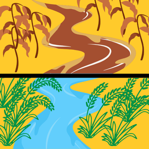
Every object reflects some wavelengths of light more or less than others. We can see this with our eyes, since, for example, plants reflect a lot of green in the summer, and then as that green diminishes in the fall they look more yellow or orange. The image below shows spectral signatures for water, soil, and vegetation:

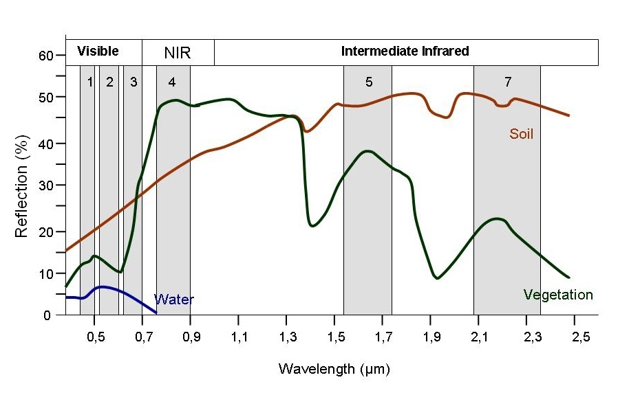> Image source: SEOS Project

Healthy vegetation reflects a lot of Near-InfraRed (NIR) radiation. Less healthy vegetation reflects a similar amounts of the visible light spectra, but less NIR radiation. We don’t see a huge drop in Green radiation until the plant is very stressed or dead. That means that NIR allows us to get ahead of what we can see with our eyes.

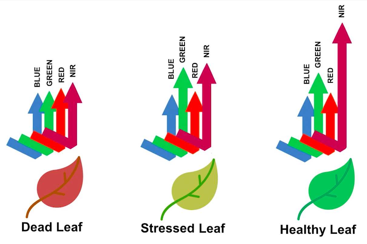Healthy leaves reflect a lot of NIR radiation compared to dead or stressed leaves > Image source: Spectral signature literature review by px39n

Different species of plants reflect different spectral signatures, but the pattern of the signatures across species and sitations is similar. NDVI compares the amount of NIR reflectance to the amount of Red reflectance, thus accounting for many of the species differences and isolating the health of the plant. The formula for calculating NDVI is:

\[NDVI = \frac{(NIR - Red)}{(NIR + Red)}\]

Read more about NDVI and other vegetation indices:

Earth Data Science data formats

In Earth Data Science, we get data in three main formats:

Data type	Descriptions	Common file formats	Python type
Time Series	The same data points (e.g. streamflow) collected multiple times over time	Tabular formats (e.g. .csv, or .xlsx)	pandas DataFrame
Vector	Points, lines, and areas (with coordinates)	Shapefile (often an archive like a `.zip` file because a Shapefile is actually a collection of at least 3 files)	geopandas GeoDataFrame
Raster	Evenly spaced spatial grid (with coordinates)	GeoTIFF (`.tif`), NetCDF (`.nc`), HDF (`.hdf`)	rioxarray DataArray

Check out the sections about about vector data and raster data in the textbook.

STEP 0: Set up

First, you can use the following parameters to change things about the workflow:

id = 'shortcourse'
site_name = 'Al Jawf Region Saudi Arabia'
project_name = 'Al Jawf Saudi Arabia Irrigation'
boundary_dir = 'al-jawf-region'
event = 'groundwater irrigation'
start_year = '2001'
end_year = '2022'
event_year = '2012'

Import libraries

We’ll need some Python libraries to complete this workflow.

Try It: Import necessary libraries

In the cell below, making sure to keep the packages in order, add packages for:

Working with DataFrames
Working with GeoDataFrames
Making interactive plots of tabular and vector data

Reflect and Respond

What are we using the rest of these packages for? See if you can figure it out as you complete the notebook.

import json
from glob import glob

import earthpy
import hvplot.xarray
import rioxarray as rxr
import xarray as xr

See our solution!

import json
from glob import glob

import earthpy
import geopandas as gpd
import hvplot.pandas
import hvplot.xarray
import pandas as pd
import rioxarray as rxr
import xarray as xr

Download sample data

In this analysis, you’ll need to download multiple data files to your computer rather than streaming them from the web. You’ll need to set up a folder for the files, and while you’re at it download the sample data there.

GOTCHA ALERT!

A lot of times in Python we say “directory” to mean a “folder” on your computer. The two words mean the same thing in this context.

Try It

In the cell below, replace ‘Project Name’ with ‘Al Jawf Saudi Arabia Irrigation and ’my-data-folder’ with a descriptive directory name.

project = earthpy.Project(
    'Project Name, dirname='my-data-folder')
project.get_data()

See our solution!

project = earthpy.Project(project_name)
project.get_data()


**Final Configuration Loaded:**
{}
🔄 Fetching metadata for article 29521241...
✅ Found 2 files for download.
Downloading from https://ndownloader.figshare.com/files/56105732
Extracted output to /home/runner/.local/share/earth-analytics/al-jawf-saudi-arabia-irrigation/al-jawf-ndvi
Downloading from https://ndownloader.figshare.com/files/56105726
Extracted output to /home/runner/.local/share/earth-analytics/al-jawf-saudi-arabia-irrigation/al-jawf-region

STEP 1: Site map

Study Area: Al Jawf Region Saudi Arabia

Reflect and Respond

For this coding challenge, we are interested in the boundary of the Al Jawf Region Saudi Arabia, and the health of vegetation in the area measured on a scale from -1 to 1. In the cell below, answer the following question: What data type do you think the boundary will be? What about the vegetation health?

Load the Al Jawf Region Saudi Arabia boundary

Try It

Locate the boundary files in your download directory
Change 'boundary-directory' to the actual location
Load the data into Python and check that it worked

# Load in the boundary data
boundary_gdf = gpd.read_file(
    project.project_dir / 'boundary-directory')
# Check that it worked

See our solution!

# Load in the boundary data
boundary_gdf = gpd.read_file(
    project.project_dir / boundary_dir)
# Check that it worked
boundary_gdf

	element	id	admin_leve	boundary	name	name_en	type	ISO3166-2	alt_name_e	alt_name_f	...	name_vi	name_war	name_wuu	name_zh	place	population	populati_1	source_pop	wikidata	geometry
0	relation	3842543	4	administrative	منطقة الجوف	Al Jawf Region	boundary	SA-12	Al-Jawf Province	Al Jawf	...	Al Jawf	Al Jawf	焦夫省	焦夫省	state	440009	2010	stats.gov.sa	Q1471266	POLYGON ((37.00617 31.50064, 37.01162 31.50183...

1 rows × 66 columns

# Plot the results with web tile images
boundary_gdf.hvplot()

See our solution!

# Plot the results with web tile images
boundary_gdf.hvplot(
    geo=True, tiles='EsriImagery',
    fill_color=None, line_color='black',
    title=site_name,
    frame_width=500)

STEP 2: Wrangle Raster Data

Load in NDVI data

Now you need to load all the downloaded files into Python. Let’s start by getting all the file names. You will also need to extract the date from the filename. Check out the lesson on getting information from filenames in the textbook.

Instead of writing out the names of all the files you want, you can use the glob utility to find all files that match a pattern formed with the wildcard character *. The wildcard can represent any string of alphanumeric characters. For example, the pattern 'file_*.tif' will match the files 'file_1.tif', 'file_2.tiv', or even 'file_qeoiurghtfoqaegbn34pf.tif'… but it will not match 'something-else.csv' or even 'something-else.tif'.

In this notebook, we’ll use the .rglob(), or recursive glob method of the Path object instead. It works similarly, but you’ll notice that we have to convert the results to a list with the list() function.

GOTCHA ALERT!

glob doesn’t necessarily find files in the order you would expect. Make sure to sort your file names like it says in the textbook.

Reflect and Respond

Take a look at the file names for the NDVI files. What do you notice is the same for all the files? Keep in mind that for this analysis you only want to import the NDVI files, not the Quality files (which would be used to identify potential incorrect measurements).

Try It

Create a pattern for the files you want to import. Your pattern should include the parts of the file names that are the same for all files, and replace the rest with the * character. Make sure to match the NDVI files, but not the Quality files!
Replace ndvi-pattern with your pattern
Run the code and make sure that you are getting all the files you want and none of the files you don’t!

# Get a sorted list of NDVI tif file paths
ndvi_paths = sorted(list(project.project_dir.rglob('ndvi-pattern')))

# Display the first and last three files paths to check the pattern
ndvi_paths[:3], ndvi_paths[-3:]

See our solution!

# Get a sorted list of NDVI tif file paths
ndvi_paths = sorted(list(project.project_dir.rglob('*NDVI*.tif')))

# Display the first and last three files paths to check the pattern
ndvi_paths[:3], ndvi_paths[-3:]

([PosixPath('/home/runner/.local/share/earth-analytics/al-jawf-saudi-arabia-irrigation/al-jawf-ndvi/MOD13Q1.061_2001137_to_2022244/MOD13Q1.061__250m_16_days_NDVI_doy2001145000000_aid0001.tif'),
  PosixPath('/home/runner/.local/share/earth-analytics/al-jawf-saudi-arabia-irrigation/al-jawf-ndvi/MOD13Q1.061_2001137_to_2022244/MOD13Q1.061__250m_16_days_NDVI_doy2001161000000_aid0001.tif'),
  PosixPath('/home/runner/.local/share/earth-analytics/al-jawf-saudi-arabia-irrigation/al-jawf-ndvi/MOD13Q1.061_2001137_to_2022244/MOD13Q1.061__250m_16_days_NDVI_doy2001177000000_aid0001.tif')],
 [PosixPath('/home/runner/.local/share/earth-analytics/al-jawf-saudi-arabia-irrigation/al-jawf-ndvi/MOD13Q1.061_2001137_to_2022244/MOD13Q1.061__250m_16_days_NDVI_doy2020177000000_aid0001.tif'),
  PosixPath('/home/runner/.local/share/earth-analytics/al-jawf-saudi-arabia-irrigation/al-jawf-ndvi/MOD13Q1.061_2001137_to_2022244/MOD13Q1.061__250m_16_days_NDVI_doy2020193000000_aid0001.tif'),
  PosixPath('/home/runner/.local/share/earth-analytics/al-jawf-saudi-arabia-irrigation/al-jawf-ndvi/MOD13Q1.061_2001137_to_2022244/MOD13Q1.061__250m_16_days_NDVI_doy2020209000000_aid0001.tif')])

Repeating tasks in Python

Now you should have a few dozen files! For each file, you need to:

Load the file in using the rioxarray library
Get the date from the file name
Add the date as a dimension coordinate
Give your data variable a name

You don’t want to write out the code for each file! That’s a recipe for copy pasta. Luckily, Python has tools for doing similar tasks repeatedly. In this case, you’ll use one called a for loop.

There’s some code below that uses a for loop in what is called an accumulation pattern to process each file. That means that you will save the results of your processing to a list each time you process the files, and then merge all the arrays in the list.

Try It

Look at the file names. How many characters from the end is the date? doy_start and doy_end are used to extract the day of the year (doy) from the file name. You will need to count characters from the end and change the values to get the right part of the file name. HINT: the index -1 in Python means the last value, -2 second-to-last, and so on.
Replace any required variable names with your chosen variable names

doy_start = -1
doy_end = -1

# Loop through each NDVI image
ndvi_das = []
for ndvi_path in ndvi_paths:
    # Get date from file name

    # Open dataset

    # Add date dimension and clean up metadata
    da = da.assign_coords({'date': date})
    da = da.expand_dims({'date': 1})
    da.name = 'NDVI'

    # Prepare for concatenation

See our solution!

doy_start = -25
doy_end = -19

# Loop through each NDVI image
ndvi_das = []
for ndvi_path in ndvi_paths:
    # Get date from the file name
    doy = ndvi_path.name[doy_start:doy_end]
    date = pd.to_datetime(doy, format='%Y%j')

    # Open dataset
    da = rxr.open_rasterio(ndvi_path, mask_and_scale=True).squeeze()

    # Add date dimension and clean up metadata
    da = da.assign_coords({'date': date})
    da = da.expand_dims({'date': 1})
    da.name = 'NDVI'

    # Prepare for concatenation
    ndvi_das.append(da)

len(ndvi_das)

Combine Rasters

Next, stack your arrays by date into a time series using the xr.combine_by_coords() function. You will have to tell it which dimension you want to stack your data in.

# Combine NDVI images from all dates

See our solution!

# Combine NDVI images from all dates
ndvi_da = xr.combine_by_coords(ndvi_das, coords=['date'])
ndvi_da

STEP 3: Plot NDVI

Try It: Plot the change in NDVI spatially

Complete the following:

Select data from before the groundwater irrigation (2001 to 2012)
Take the temporal mean (over the date, not spatially)
Get the NDVI variable (should be a DataArray, not a Dataset)
Repeat for the data from after the groundwater irrigation (2012 to 2022)
Subtract the pre-event data from the post-event data
Plot the result using a diverging color map like cmap=plt.cm.PiYG

There are different types of color maps for different types of data. In this case, we want decreases to be a different color from increases, so we should use a diverging color map. Check out available colormaps in the matplotlib documentation.

Looking for an Extra Challenge?

For an extra challenge, add the Al Jawf Region Saudi Arabia boundary to the plot.

# Compute the difference in NDVI before and after

# Plot the difference
(
    ndvi_diff.hvplot(x='', y='', cmap='', geo=True)
    *
    gdf.hvplot(geo=True, fill_color=None, line_color='black')
)

See our solution!

ndvi_diff = (
    ndvi_da
        .sel(date=slice(event_year, end_year))
        .mean('date')
        .NDVI 
   - ndvi_da
        .sel(date=slice(start_year, event_year))
        .mean('date')
        .NDVI
)
(
    ndvi_diff.hvplot(x='x', y='y', cmap='PiYG', geo=True)
    *
    boundary_gdf.hvplot(geo=True, fill_color=None, line_color='black')
)

STEP 4: Is the NDVI different after the groundwater irrigation?

You will apply an NDVI threshold and determine how many pixels have healthy vegetation. You can then look at the growth of vegetation over time.

Try It

Apply an NDVI threshold to identify pixels with healthy vegetation
Check that your threshold worked

# Apply NDVI threshold

See our solution!

# Create a composite of NDVI values for each year
composite_da = (
    ndvi_da
    .groupby('date.year')
    .mean(dim=['date'])
)

Now, add up the number of pixels with healthy vegetation plot that over time.

# Plot difference inside and outside the boundary

See our solution!

# Count number of vegetated pixels each year
annual_veg_da = (
    composite_da
    # Identify vegetated pixels
    .where(composite_da>0.3)
    # Count pixels in each annual image
    .count(dim=['x', 'y'])
)
annual_veg_da

Finally, plot your DataFrame. What do you observe? Don’t forget to write a headline and description of your plot!

# Plot number of vegetated pixels over time

See our solution!

# Plot number of vegetated pixels over time
(
    annual_veg_da
    .NDVI
    .hvplot(
        title=f'Vegetation over time in {site_name}',
        ylabel='Vegetated pixels',
        xlabel='Year')
)