%%bash
find ~/earth-analytics/data/species-distribution -name '*.shp' /home/runner/earth-analytics/data/species-distribution/wwf_ecoregions/wwf_ecoregions.shpIntroduction to vector data operations
Tasiyagnunpa (or Western Meadowlark, or sturnella neglecta) migrates each year to nest on the Great Plains in the United States. Using crowd-sourced observations of these birds, we can see that migration happening throughout the year.
Read more about the Lakota connection to Tasiyagnunpa from Native Sun News Today
Reflect on what you know about migration. You could consider:
In the imports cell, we’ve included a number of packages that you will need. Add imports for packages that will help you:
import os
import pathlibimport os
import pathlib
import geopandas as gpd
import pandas as pdFor this challenge, you will need to save some data to the computer you’re working on. We suggest saving to somewhere in your home folder (e.g. /home/username), rather than to your GitHub repository, since data files can easily become too large for GitHub.
The home directory is different for every user! Your home directory probably won’t exist on someone else’s computer. Make sure to use code like pathlib.Path.home() to compute the home directory on the computer the code is running on. This is key to writing reproducible and interoperable code.
The code below will help you get started with making a project directory
'your-project-directory-name-here' and 'your-gbif-data-directory-name-here' with descriptive namesls ~/earth-analytics/data# Create data directory in the home folder
data_dir = os.path.join(
# Home directory
pathlib.Path.home(),
# Earth analytics data directory
'earth-analytics',
'data',
# Project directory
'your-project-directory-name-here',
)
os.makedirs(data_dir, exist_ok=True)# Create data directory in the home folder
data_dir = os.path.join(
pathlib.Path.home(),
'earth-analytics',
'data',
'species-distribution',
)
os.makedirs(data_dir, exist_ok=True)Track observations of Taciyagnunpa across different ecoregions! You should be able to see changes in the number of observations in each ecoregion throughout the year.
The ecoregion data will be available as a shapefile. Learn more about shapefiles and vector data in this Introduction to Spatial Vector Data File Formats in Open Source Python
The ecoregion boundaries take some time to download – they come in at about 150MB. To use your time most efficiently, we recommend caching the ecoregions data on the machine you’re working on so that you only have to download once. To do that, we’ll also introduce the concept of conditionals, or code that adjusts what it does based on the situation.
Read more about conditionals in this Intro Conditional Statements in Python
your/url/here with the URL you found, making sure to format it so it is easily readable. Also, replace ecoregions_dirname and ecoregions_filename with descriptive and machine-readable names for your project’s file structure.# Set up the ecoregion boundary URL
url = "your/url/here"
# Set up a path to save the data on your machine
the_dir = os.path.join(project_data_dir, 'ecoregions_dirname')
# Make the ecoregions directory
# Join ecoregions shapefile path
a_path = os.path.join(the_dir, 'ecoregions_filename.shp')
# Only download once
if not os.path.exists(a_path):
my_gdf = gpd.read_file(your_url_here)
my_gdf.to_file(your_path_here)# Set up the ecoregion boundary URL
ecoregions_url = (
"https://storage.googleapis.com/teow2016/Ecoregions2017.zip")
# Set up a path to save the data on your machine
ecoregions_dir = os.path.join(data_dir, 'wwf_ecoregions')
os.makedirs(ecoregions_dir, exist_ok=True)
ecoregions_path = os.path.join(ecoregions_dir, 'wwf_ecoregions.shp')
# Only download once
if not os.path.exists(ecoregions_path):
ecoregions_gdf = gpd.read_file(ecoregions_url)
ecoregions_gdf.to_file(ecoregions_path)Let’s check that that worked! To do so we’ll use a bash command called find to look for all the files in your project directory with the .shp extension:
%%bash
find ~/earth-analytics/data/species-distribution -name '*.shp' /home/runner/earth-analytics/data/species-distribution/wwf_ecoregions/wwf_ecoregions.shpYou can also run bash commands in the terminal!
Learn more about bash in this Introduction to Bash
Download and save ecoregion boundaries from the EPA:
a_path with the path your created for your ecoregions file.GeoDataFrame easier to work with. Many of the same methods you learned for pandas DataFrames are the same for GeoDataFrames! NOTE: Make sure to keep the 'SHAPE_AREA' column around – we will need that later!.plot() to make sure the download worked.# Open up the ecoregions boundaries
gdf = gpd.read_file(a_path)
# Name the index so it will match the other data later on
gdf.index.name = 'ecoregion'
# Plot the ecoregions to check download--------------------------------------------------------------------------- NameError Traceback (most recent call last) Cell In[5], line 2 1 # Open up the ecoregions boundaries ----> 2 gdf = gpd.read_file(a_path) 4 # Name the index so it will match the other data later on 5 gdf.index.name = 'ecoregion' NameError: name 'a_path' is not defined
# Open up the ecoregions boundaries
ecoregions_gdf = (
gpd.read_file(ecoregions_path)
.rename(columns={
'ECO_NAME': 'name',
'SHAPE_AREA': 'area'})
[['name', 'area', 'geometry']]
)
# We'll name the index so it will match the other data
ecoregions_gdf.index.name = 'ecoregion'
# Plot the ecoregions to check download
ecoregions_gdf.plot(edgecolor='black', color='skyblue')ERROR 1: PROJ: proj_create_from_database: Open of /usr/share/miniconda/envs/learning-portal/share/proj failed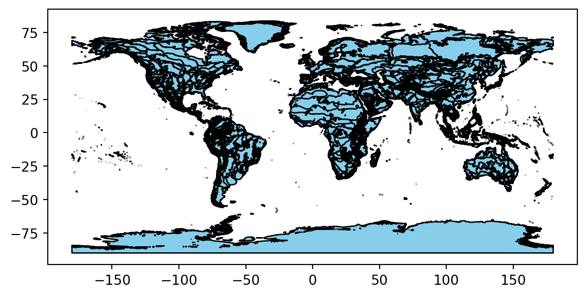
For this challenge, you will use a database called the Global Biodiversity Information Facility (GBIF). GBIF is compiled from species observation data all over the world, and includes everything from museum specimens to photos taken by citizen scientists in their backyards. We’ve compiled some sample data in the same format that you will get from GBIF.
gbif_url. You can get sample data from https://github.com/cu-esiil-edu/esiil-learning-portal/releases/download/data-release/species-distribution-foundations-data.zip# Load the GBIF data
gbif_df = pd.read_csv(
gbif_url,
delimiter='\t',
index_col='gbifID',
usecols=['gbifID', 'decimalLatitude', 'decimalLongitude', 'month'])
gbif_df.head()--------------------------------------------------------------------------- NameError Traceback (most recent call last) Cell In[7], line 3 1 # Load the GBIF data 2 gbif_df = pd.read_csv( ----> 3 gbif_url, 4 delimiter='\t', 5 index_col='gbifID', 6 usecols=['gbifID', 'decimalLatitude', 'decimalLongitude', 'month']) 7 gbif_df.head() NameError: name 'gbif_url' is not defined
# Define the download URL
gbif_url = (
"https://github.com/cu-esiil-edu/esiil-learning-portal/releases/download"
"/data-release/species-distribution-foundations-data.zip")
# Set up a path to save the data on your machine
gbif_dir = os.path.join(data_dir, 'gbif_veery')
os.makedirs(gbif_dir, exist_ok=True)
gbif_path = os.path.join(gbif_dir, 'gbif_veery.zip')
# Only download once
if not os.path.exists(gbif_path):
# Load the GBIF data
gbif_df = pd.read_csv(
gbif_url,
delimiter='\t',
index_col='gbifID',
usecols=['gbifID', 'decimalLatitude', 'decimalLongitude', 'month'])
# Save the GBIF data
gbif_df.to_csv(gbif_path, index=False)
gbif_df = pd.read_csv(gbif_path)
gbif_df.head()| decimalLatitude | decimalLongitude | month | |
|---|---|---|---|
| 0 | 40.771550 | -73.97248 | 9 |
| 1 | 42.588123 | -85.44625 | 5 |
| 2 | 43.703064 | -72.30729 | 5 |
| 3 | 48.174270 | -77.73126 | 7 |
| 4 | 42.544277 | -72.44836 | 5 |
To plot the GBIF data, we need to convert it to a GeoDataFrame first. This will make some special geospatial operations from geopandas available, such as spatial joins and plotting.
your_dataframe with the name of the DataFrame you just got from GBIFlongitude_column_name and latitude_column_name with column names from your `DataFrameGeoDataFrame of the GBIF data.gbif_gdf = (
gpd.GeoDataFrame(
your_dataframe,
geometry=gpd.points_from_xy(
your_dataframe.longitude_column_name,
your_dataframe.latitude_column_name),
crs="EPSG:4326")
# Select the desired columns
[[]]
)
gbif_gdfgbif_gdf = (
gpd.GeoDataFrame(
gbif_df,
geometry=gpd.points_from_xy(
gbif_df.decimalLongitude,
gbif_df.decimalLatitude),
crs="EPSG:4326")
# Select the desired columns
[['month', 'geometry']]
)
gbif_gdf| month | geometry | |
|---|---|---|
| 0 | 9 | POINT (-73.97248 40.77155) |
| 1 | 5 | POINT (-85.44625 42.58812) |
| 2 | 5 | POINT (-72.30729 43.70306) |
| 3 | 7 | POINT (-77.73126 48.17427) |
| 4 | 5 | POINT (-72.44836 42.54428) |
| ... | ... | ... |
| 162770 | 5 | POINT (-78.75946 45.0954) |
| 162771 | 7 | POINT (-88.02332 48.99255) |
| 162772 | 5 | POINT (-72.79677 43.46352) |
| 162773 | 6 | POINT (-81.32435 46.04416) |
| 162774 | 5 | POINT (-73.82481 40.61684) |
162775 rows × 2 columns
Much of the data in GBIF is crowd-sourced. As a result, we need not just the number of observations in each ecosystem each month – we need to normalize by some measure of sampling effort. After all, we wouldn’t expect the same number of observations in the Arctic as we would in a National Park, even if there were the same number of Veeries. In this case, we’re normalizing using the average number of observations for each ecosystem and each month. This should help control for the number of active observers in each location and time of year.
First things first – let’s load your stored variables.
%store -rYou can combine the ecoregions and the observations spatially using a method called .sjoin(), which stands for spatial join.
Check out the geopandas documentation on spatial joins to help you figure this one out. You can also ask your favorite LLM (Large-Language Model, like ChatGPT)
how= and predicate= parameters of the spatial join.gbif_ecoregion_gdf = (
ecoregions_gdf
# Match the CRS of the GBIF data and the ecoregions
.to_crs(gbif_gdf.crs)
# Find ecoregion for each observation
.sjoin(
gbif_gdf,
how='',
predicate='')
# Select the required columns
)
gbif_ecoregion_gdfgbif_ecoregion_gdf = (
ecoregions_gdf
# Match the CRS of the GBIF data and the ecoregions
.to_crs(gbif_gdf.crs)
# Find ecoregion for each observation
.sjoin(
gbif_gdf,
how='inner',
predicate='contains')
# Select the required columns
[['month', 'name']]
)
gbif_ecoregion_gdf| month | name | |
|---|---|---|
| ecoregion | ||
| 12 | 5 | Alberta-British Columbia foothills forests |
| 12 | 5 | Alberta-British Columbia foothills forests |
| 12 | 6 | Alberta-British Columbia foothills forests |
| 12 | 7 | Alberta-British Columbia foothills forests |
| 12 | 6 | Alberta-British Columbia foothills forests |
| ... | ... | ... |
| 839 | 10 | North Atlantic moist mixed forests |
| 839 | 9 | North Atlantic moist mixed forests |
| 839 | 9 | North Atlantic moist mixed forests |
| 839 | 9 | North Atlantic moist mixed forests |
| 839 | 9 | North Atlantic moist mixed forests |
159537 rows × 2 columns
columns_to_group_by with a list of columns. Keep in mind that you will end up with one row for each group – you want to count the observations in each ecoregion by month..groupby() and .mean() methods to compute the mean occurrences by ecoregion and by month.occurrence_df = (
gbif_ecoregion_gdf
# For each ecoregion, for each month...
.groupby(columns_to_group_by)
# ...count the number of occurrences
.agg(occurrences=('name', 'count'))
)
# Get rid of rare observations (possible misidentification?)
occurrence_df = occurrence_df[...]
# Take the mean by ecoregion
mean_occurrences_by_ecoregion = (
occurrence_df
...
)
# Take the mean by month
mean_occurrences_by_month = (
occurrence_df
...
)occurrence_df = (
gbif_ecoregion_gdf
# For each ecoregion, for each month...
.groupby(['ecoregion', 'month'])
# ...count the number of occurrences
.agg(occurrences=('name', 'count'))
)
# Get rid of rare observation noise (possible misidentification?)
occurrence_df = occurrence_df[occurrence_df.occurrences>1]
# Take the mean by ecoregion
mean_occurrences_by_ecoregion = (
occurrence_df
.groupby(['ecoregion'])
.mean()
)
# Take the mean by month
mean_occurrences_by_month = (
occurrence_df
.groupby(['month'])
.mean()
)# Normalize by space and time for sampling effort
occurrence_df['norm_occurrences'] = (
occurrence_df
...
)
occurrence_dfoccurrence_df['norm_occurrences'] = (
occurrence_df
/ mean_occurrences_by_ecoregion
/ mean_occurrences_by_month
)
occurrence_df| occurrences | norm_occurrences | ||
|---|---|---|---|
| ecoregion | month | ||
| 12 | 5 | 2 | 0.000828 |
| 6 | 2 | 0.000960 | |
| 7 | 2 | 0.001746 | |
| 16 | 4 | 2 | 0.000010 |
| 5 | 2980 | 0.001732 | |
| ... | ... | ... | ... |
| 833 | 7 | 293 | 0.002173 |
| 8 | 40 | 0.001030 | |
| 9 | 11 | 0.000179 | |
| 839 | 9 | 25 | 0.005989 |
| 10 | 7 | 0.013328 |
308 rows × 2 columns
First thing first – let’s load your stored variables and import libraries.
%store -r ecoregions_gdf occurrence_dfIn the imports cell, we’ve included some packages that you will need. Add imports for packages that will help you:
# Get month names
import calendar
# Libraries for Dynamic mapping
import cartopy.crs as ccrs
import panel as pn# Get month names
import calendar
# Libraries for Dynamic mapping
import cartopy.crs as ccrs
import hvplot.pandas
import panel as pnGeoDataFrame for plottingPlotting larger files can be time consuming. The code below will streamline plotting with hvplot by simplifying the geometry, projecting it to a Mercator projection that is compatible with geoviews, and cropping off areas in the Arctic.
Download and save ecoregion boundaries from the EPA:
.simplify(.05), and save it back to the geometry column..to_crs(ccrs.Mercator())gdf to YOUR GeoDataFrame name.# Simplify the geometry to speed up processing
# Change the CRS to Mercator for mapping
# Check that the plot runs in a reasonable amount of time
gdf.hvplot(geo=True, crs=ccrs.Mercator())# Simplify the geometry to speed up processing
ecoregions_gdf.geometry = ecoregions_gdf.simplify(
.05, preserve_topology=False)
# Change the CRS to Mercator for mapping
ecoregions_gdf = ecoregions_gdf.to_crs(ccrs.Mercator())
# Check that the plot runs
ecoregions_gdf.hvplot(geo=True, crs=ccrs.Mercator())column_name_used_for_ecoregion_color and column_name_used_for_slider with the column names you wish to use.Your plot will probably still change months very slowly in your Jupyter notebook, because it calculates each month’s plot as needed. Open up the saved HTML file to see faster performance!
# Join the occurrences with the plotting GeoDataFrame
occurrence_gdf = ecoregions_gdf.join(occurrence_df)
# Get the plot bounds so they don't change with the slider
xmin, ymin, xmax, ymax = occurrence_gdf.total_bounds
# Plot occurrence by ecoregion and month
migration_plot = (
occurrence_gdf
.hvplot(
c=column_name_used_for_shape_color,
groupby=column_name_used_for_slider,
# Use background tiles
geo=True, crs=ccrs.Mercator(), tiles='CartoLight',
title="Your Title Here",
xlim=(xmin, xmax), ylim=(ymin, ymax),
frame_height=600,
widget_location='bottom'
)
)
# Save the plot
migration_plot.save('migration.html', embed=True)
# Show the plot
migration_plot# Join the occurrences with the plotting GeoDataFrame
occurrence_gdf = ecoregions_gdf.join(occurrence_df)
# Get the plot bounds so they don't change with the slider
xmin, ymin, xmax, ymax = occurrence_gdf.total_bounds
# Define the slider widget
slider = pn.widgets.DiscreteSlider(
name='month',
options={calendar.month_name[i]: i for i in range(1, 13)}
)
# Plot occurrence by ecoregion and month
migration_plot = (
occurrence_gdf
.hvplot(
c='norm_occurrences',
groupby='month',
# Use background tiles
geo=True, crs=ccrs.Mercator(), tiles='CartoLight',
title="Veery migration",
xlim=(xmin, xmax), ylim=(ymin, ymax),
frame_height=600,
colorbar=False,
widgets={'month': slider},
widget_location='bottom'
)
)
# Save the plot (if possible)
try:
migration_plot.save('migration.html', embed=True)
except Exception as exc:
print('Could not save the migration plot due to the following error:')
print(exc)
# Show the plot
migration_plot 0%| | 0/12 [00:00<?, ?it/s] 8%|▊ | 1/12 [00:00<00:01, 6.91it/s] 17%|█▋ | 2/12 [00:00<00:01, 6.23it/s] 25%|██▌ | 3/12 [00:00<00:03, 2.62it/s] 33%|███▎ | 4/12 [00:01<00:03, 2.08it/s] 42%|████▏ | 5/12 [00:02<00:03, 2.03it/s] 50%|█████ | 6/12 [00:02<00:02, 2.04it/s] 58%|█████▊ | 7/12 [00:03<00:02, 1.95it/s] 67%|██████▋ | 8/12 [00:03<00:02, 1.70it/s] 75%|███████▌ | 9/12 [00:04<00:01, 1.80it/s] 83%|████████▎ | 10/12 [00:04<00:00, 2.31it/s] 92%|█████████▏| 11/12 [00:04<00:00, 2.77it/s]100%|██████████| 12/12 [00:04<00:00, 3.24it/s] WARNING:bokeh.core.validation.check:W-1005 (FIXED_SIZING_MODE): 'fixed' sizing mode requires width and height to be set: figure(id='p19289', ...)