id = 'stars'
project_title = 'Tasiyagnunpa Migration 2023'
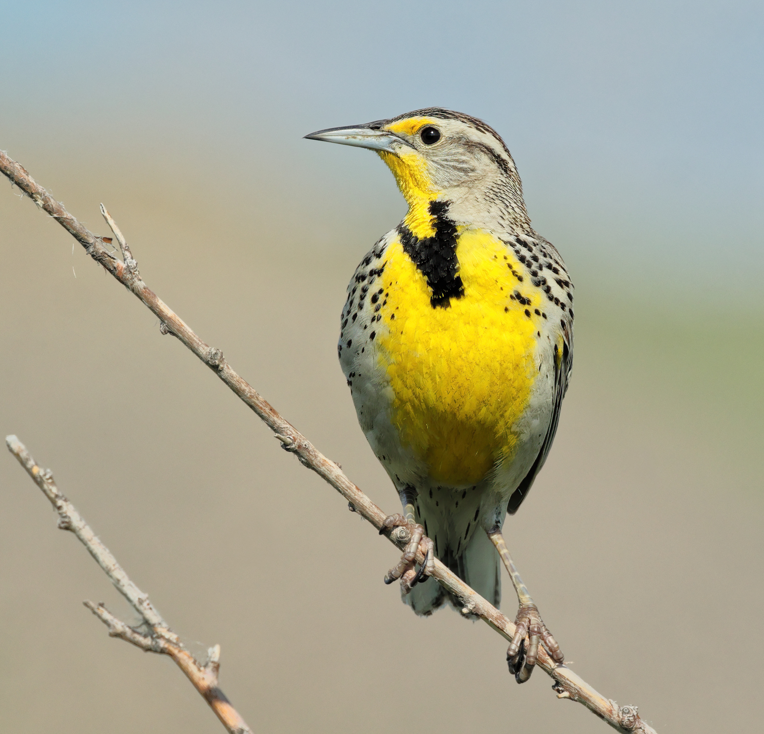
species_name = 'Tasiyagnunpa'
species_lookup = 'sturnella neglecta'
species_key = 9596413
year = 2023
gbif_filename = 'gbif_tasiyagnunpa.csv'
ecoregions_dir = 'wwf_ecoregions'
plot_filename = 'tasiyagnunpa_migration'
plot_height = 500Spring returns to the Great Plains
Mapping Tasiyagnunpa migration
Tasiyagnunpa (or Western Meadowlark, or sturnella neglecta) migrates each year to nest on the Great Plains in the United States. Using crowd-sourced observations of these birds, we can see that migration happening throughout the year. In the process, you’’ll learn about an important type of geospatial data called vector data, which records where points, lines, and shapes on the Earth.
Learning Goals:
- Combine different types of vector data with spatial joins
- Normalize species observation data to avoid collection biases
- Create a chloropleth plot
- Build an interactive display showing observation distributions over time
Tasiyagnunpa (or Western Meadowlark, or sturnella neglecta) migrates each year to nest on the Great Plains in the United States. Using crowd-sourced observations of these birds, we can see that migration happening throughout the year.
Read More
Read more about the Lakota connection to Tasiyagnunpa from Native Sun News Today
Check out our demo video!
Reflect on what you know about migration. You could consider:
- What are some reasons that animals migrate?
- How might climate change affect animal migrations?
- Do you notice any animal migrations in your area?
Before we get started, let’s define some parameters for the workflow. We’ll use these throughout to customize the workflow for this species:
STEP 1: Set up your reproducible workflow
Import Python libraries
Try It: Import packages
In the imports cell, we’ve included some packages that you will need. Add imports for packages that will help you:
- Work with tabular data
- Work with geospatial vector data
import os
import pathlib
import earthpySee our solution!
import os
import pathlib
import earthpy
import geopandas as gpd
import pandas as pdCreate a directory for your data
For this challenge, you will need to download some data to the computer you’re working on. We suggest using the earthpy library we develop to manage your downloads, since it encapsulates many best practices as far as:
- Where to store your data
- Dealing with archived data like .zip files
- Avoiding version control problems
- Making sure your code works cross-platform
- Avoiding duplicate downloads
If you’re working on one of our assignments through GitHub Classroom, it also lets us build in some handy defaults so that you can see your data files while you work.
Try It: Create a project folder
The code below will help you get started with making a project directory
- Replace
'your-project-directory-name-here'with a descriptive name - Run the cell
- The code should have printed out the path to your data files. Check that your data directory exists and has data in it using the terminal or your Finder/File Explorer.
File structure
These days, a lot of people find your file by searching for them or selecting from a Bookmarks or Recents list. Even if you don’t use it, your computer also keeps files in a tree structure of folders. Put another way, you can organize and find files by travelling along a unique path, e.g. My Drive > Documents > My awesome project > A project file where each subsequent folder is inside the previous one. This is convenient because all the files for a project can be in the same place, and both people and computers can rapidly locate files they want, provided they remember the path.
You may notice that when Python prints out a file path like this, the folder names are separated by a / or \ (depending on your operating system). This character is called the file separator, and it tells you that the next piece of the path is inside the previous one.
# Create data directory
project = earthpy.Project(
title=project_title,
dirname='your-project-directory-name-here')
# Download sample data
project.get_data()
# Display the project directory
project.project_dirSee our solution!
# Create data directory
project = earthpy.Project(title=project_title)
# Download sample data
project.get_data()
# Display the project directory
project.project_dir
**Final Configuration Loaded:**
{}
🔄 Fetching metadata for article 29119190...
✅ Found 2 files for download.
[('https://ndownloader.figshare.com/files/54711704', 'gbif_tasiyagnunpa.csv', 'file'), ('https://ndownloader.figshare.com/files/54711734', 'wwf_ecoregions', 'zip')]
gbif_tasiyagnunpa.csv
Downloading from https://ndownloader.figshare.com/files/54711704
[PosixPath('/home/runner/.local/share/earth-analytics/tasiyagnunpa-migration-2023/gbif_tasiyagnunpa.csv')]
wwf_ecoregions
Downloading from https://ndownloader.figshare.com/files/54711734
Extracted output to /home/runner/.local/share/earth-analytics/tasiyagnunpa-migration-2023/wwf_ecoregions
[PosixPath('/home/runner/.local/share/earth-analytics/tasiyagnunpa-migration-2023/gbif_tasiyagnunpa.csv'), PosixPath('/home/runner/.local/share/earth-analytics/tasiyagnunpa-migration-2023/wwf_ecoregions')]PosixPath('/home/runner/.local/share/earth-analytics/tasiyagnunpa-migration-2023')STEP 2: Define your study area – the ecoregions of North America
Your sample data package included a Shapefile of global ecoregions. You should be able to see changes in the number of observations of Tasiyagnunpa in each ecoregion throughout the year.
You don’t have to use ecoregions to group species observations – you could choose to use political boundaries like countries or states, other natural boundaries like watersheds, or even uniform hexagonal areas as is common in conservation work. We chose ecoregions because we expect the suitability for a species at a particular time of year to be relatively consistent across the region.
Read More
The ecoregion data will be available as a shapefile. Learn more about shapefiles and vector data in this Introduction to Spatial Vector Data File Formats in Open Source Python
Load the ecoregions into Python
Try It: Load ecoregions into Python
Download and save ecoregion boundaries from the EPA:
- Replace
a_pathwith the path your created for your ecoregions file. - (optional) Consider renaming and selecting columns to make your
GeoDataFrameeasier to work with. Many of the same methods you learned forpandasDataFrames are the same forGeoDataFrames! NOTE: Make sure to keep the'SHAPE_AREA'column around – we will need that later! - Make a quick plot with
.plot()to make sure the download worked. - Run the cell to load the data into Python
# Open up the ecoregions boundaries
gdf = gpd.read_file(a_path)
# Name the index so it will match the other data later on
gdf.index.name = 'ecoregion'
# Plot the ecoregions quickly to check downloadSee our solution!
# Open up the ecoregions boundaries
ecoregions_gdf = (
gpd.read_file(project.project_dir / ecoregions_dir)
.rename(columns={
'ECO_NAME': 'name',
'SHAPE_AREA': 'area'})
[['name', 'area', 'geometry']]
)
# We'll name the index so it will match the other data
ecoregions_gdf.index.name = 'ecoregion'
# Plot the ecoregions quickly to check download
ecoregions_gdf.plot(edgecolor='black', color='skyblue')ERROR 1: PROJ: proj_create_from_database: Open of /usr/share/miniconda/envs/learning-portal/share/proj failed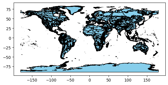
STEP 3: Load species observation data
For this challenge, you will use a database called the Global Biodiversity Information Facility (GBIF). GBIF is compiled from species observation data all over the world, and includes everything from museum specimens to photos taken by citizen scientists in their backyards. We’ve compiled some sample data in the same format that you will get from GBIF.
Let’s start by looking at a little of the raw data.
gbif_path = project.project_dir / gbif_filename
Try It: Load GBIF data
- Look at the beginning of the file you downloaded using the code below. What do you think the delimiter is?
- Run the following code cell. What happens?
- Uncomment and modify the parameters of
pd.read_csv()below until your data loads successfully and you have only the columns you want.
You can use the following code to look at the beginning of your file:
!head -n 2 $gbif_path gbifID datasetKey occurrenceID kingdom phylum class order family genus species infraspecificEpithet taxonRank scientificName verbatimScientificName verbatimScientificNameAuthorship countryCode locality stateProvince occurrenceStatus individualCount publishingOrgKey decimalLatitude decimalLongitude coordinateUncertaintyInMeters coordinatePrecision elevation elevationAccuracy depth depthAccuracy eventDate day month year taxonKey speciesKey basisOfRecord institutionCode collectionCode catalogNumber recordNumber identifiedBy dateIdentified license rightsHolder recordedBy typeStatus establishmentMeans lastInterpreted mediaType issue
4501319588 2f54cb88-4167-499a-81fb-0a2d02465212 http://arctos.database.museum/guid/DMNS:Bird:57539?seid=6172480 Animalia Chordata Aves Passeriformes Icteridae Sturnella Sturnella neglecta SPECIES Sturnella neglecta Audubon, 1844 Sturnella neglecta US Fort Collins, 6888 East County Road 56 Colorado PRESENT a2ef6dd1-8886-48c9-8025-c62bac973cc7 40.657779 -104.94913 80.0 1609.0 0.0 2023-05-30 30 5 2023 9596413 9596413 PRESERVED_SPECIMEN DMNS Bird DMNS:Bird:57539 Greenwood Wildlife Rehabilitation Center 2023-05-30T00:00:00 CC_BY_NC_4_0 Collector(s): Greenwood Wildlife Rehabilitation Center 2025-02-06T17:47:06.161Z COORDINATE_ROUNDED;CONTINENT_DERIVED_FROM_COORDINATES;INSTITUTION_MATCH_FUZZY;COLLECTION_MATCH_FUZZY# Load the GBIF data
gbif_df = pd.read_csv(
gbif_path,
delimiter='',
index_col='',
usecols=[]
)
gbif_df.head()See our solution!
# Load the GBIF data
gbif_df = pd.read_csv(
gbif_path,
delimiter='\t',
index_col='gbifID',
usecols=['gbifID', 'decimalLatitude', 'decimalLongitude', 'month'])
gbif_df.head()| decimalLatitude | decimalLongitude | month | |
|---|---|---|---|
| gbifID | |||
| 4501319588 | 40.657779 | -104.949130 | 5 |
| 4501319649 | 40.266835 | -105.163977 | 7 |
| 4697139297 | 31.569170 | -109.700950 | 2 |
| 4735897257 | 40.582947 | -102.277350 | 4 |
| 4719794206 | 39.266953 | -104.515920 | 6 |
Convert the GBIF data to a GeoDataFrame
To plot the GBIF data, we need to convert it to a GeoDataFrame first. This will make some special geospatial operations from geopandas available, such as spatial joins and plotting.
Try It: Convert `DataFrame` to `GeoDataFrame`
- Replace
your_dataframewith the name of theDataFrameyou just got from GBIF - Replace
longitude_column_nameandlatitude_column_namewith column names from your `DataFrame - Run the code to get a
GeoDataFrameof the GBIF data.
gbif_gdf = (
gpd.GeoDataFrame(
your_dataframe,
geometry=gpd.points_from_xy(
your_dataframe.longitude_column_name,
your_dataframe.latitude_column_name),
crs="EPSG:4326")
# Select the desired columns
[[]]
)
gbif_gdfSee our solution!
gbif_gdf = (
gpd.GeoDataFrame(
gbif_df,
geometry=gpd.points_from_xy(
gbif_df.decimalLongitude,
gbif_df.decimalLatitude),
crs="EPSG:4326")
# Select the desired columns
[['month', 'geometry']]
)
gbif_gdf| month | geometry | |
|---|---|---|
| gbifID | ||
| 4501319588 | 5 | POINT (-104.94913 40.65778) |
| 4501319649 | 7 | POINT (-105.16398 40.26684) |
| 4697139297 | 2 | POINT (-109.70095 31.56917) |
| 4735897257 | 4 | POINT (-102.27735 40.58295) |
| 4719794206 | 6 | POINT (-104.51592 39.26695) |
| ... | ... | ... |
| 4796460466 | 4 | POINT (-118.89593 35.43725) |
| 4720342585 | 4 | POINT (-109.28928 40.43625) |
| 4725888708 | 6 | POINT (-111.30072 47.66419) |
| 4512646405 | 7 | POINT (-109.53653 50.8687) |
| 5028881325 | 4 | POINT (-106.66021 52.12968) |
249939 rows × 2 columns
STEP 4: Count the number of observations in each ecosystem, during each month of 2023
Much of the data in GBIF is crowd-sourced. As a result, we need not just the number of observations in each ecosystem each month – we need to normalize by some measure of sampling effort. After all, we wouldn’t expect the same number of observations at the North Pole as we would in a National Park, even if there were the same number organisms. In this case, we’re normalizing using the average number of observations for each ecosystem and each month. This should help control for the number of active observers in each location and time of year.
Identify the ecoregion for each observation
You can combine the ecoregions and the observations spatially using a method called .sjoin(), which stands for spatial join.
Read More
Check out the geopandas documentation on spatial joins to help you figure this one out. You can also ask your favorite LLM (Large-Language Model, like ChatGPT)
Try It: Perform a spatial join
- Identify the correct values for the
how=andpredicate=parameters of the spatial join. - Select only the columns you will need for your plot.
- Run the code.
gbif_ecoregion_gdf = (
ecoregions_gdf
# Match the CRS of the GBIF data and the ecoregions
.to_crs(gbif_gdf.crs)
# Find ecoregion for each observation
.sjoin(
gbif_gdf,
how='',
predicate='')
# Select the required columns
)
gbif_ecoregion_gdfSee our solution!
gbif_ecoregion_gdf = (
ecoregions_gdf
# Match the CRS of the GBIF data and the ecoregions
.to_crs(gbif_gdf.crs)
# Find ecoregion for each observation
.sjoin(
gbif_gdf,
how='inner',
predicate='contains')
# Select the required columns
[['month', 'name']]
)
gbif_ecoregion_gdf| month | name | |
|---|---|---|
| ecoregion | ||
| 12 | 6 | Alberta-British Columbia foothills forests |
| 12 | 6 | Alberta-British Columbia foothills forests |
| 12 | 6 | Alberta-British Columbia foothills forests |
| 12 | 6 | Alberta-British Columbia foothills forests |
| 12 | 6 | Alberta-British Columbia foothills forests |
| ... | ... | ... |
| 833 | 6 | Northern Rockies conifer forests |
| 833 | 6 | Northern Rockies conifer forests |
| 833 | 6 | Northern Rockies conifer forests |
| 833 | 5 | Northern Rockies conifer forests |
| 833 | 5 | Northern Rockies conifer forests |
248940 rows × 2 columns
Count the observations in each ecoregion each month
Try It: Group observations by ecoregion
- Replace
columns_to_group_bywith a list of columns. Keep in mind that you will end up with one row for each group – you want to count the observations in each ecoregion by month. - Select only month/ecosystem combinations that have more than one occurrence recorded, since a single occurrence could be an error.
- Use the
.groupby()and.mean()methods to compute the mean occurrences by ecoregion and by month. - Run the code – it will normalize the number of occurrences by month and ecoretion.
occurrence_df = (
gbif_ecoregion_gdf
# For each ecoregion, for each month...
.groupby(columns_to_group_by)
# ...count the number of occurrences
.agg(occurrences=('name', 'count'))
)
# Get rid of rare observations (possible misidentification?)
occurrence_df = occurrence_df[...]
# Take the mean by ecoregion
mean_occurrences_by_ecoregion = (
occurrence_df
...
)
# Take the mean by month
mean_occurrences_by_month = (
occurrence_df
...
)See our solution!
occurrence_df = (
gbif_ecoregion_gdf
# For each ecoregion, for each month...
.groupby(['ecoregion', 'month'])
# ...count the number of occurrences
.agg(occurrences=('name', 'count'))
)
# Get rid of rare observation noise (possible misidentification?)
occurrence_df = occurrence_df[occurrence_df.occurrences>1]
# Take the mean by ecoregion
mean_occurrences_by_ecoregion = (
occurrence_df
.groupby(['ecoregion'])
.mean()
)
# Take the mean by month
mean_occurrences_by_month = (
occurrence_df
.groupby(['month'])
.mean()
)Normalize the observations
Try It: Normalize
- Divide occurrences by the mean occurrences by month AND the mean occurrences by ecoregion
# Normalize by space and time for sampling effort
occurrence_df['norm_occurrences'] = (
occurrence_df
...
)
occurrence_dfSee our solution!
occurrence_df['norm_occurrences'] = (
occurrence_df
/ mean_occurrences_by_ecoregion
/ mean_occurrences_by_month
)
occurrence_df| occurrences | norm_occurrences | ||
|---|---|---|---|
| ecoregion | month | ||
| 12 | 4 | 5 | 0.000715 |
| 5 | 22 | 0.001941 | |
| 6 | 46 | 0.005814 | |
| 7 | 5 | 0.001261 | |
| 8 | 4 | 0.001995 | |
| ... | ... | ... | ... |
| 833 | 8 | 114 | 0.002137 |
| 9 | 166 | 0.002584 | |
| 10 | 75 | 0.000989 | |
| 11 | 7 | 0.000084 | |
| 12 | 5 | 0.000055 |
679 rows × 2 columns
STEP 5: Plot the Tasiyagnunpa observations by month
First thing first – let’s load your stored variables and import libraries.
%store -r ecoregions_gdf occurrence_df
Try It: Import packages
In the imports cell, we’ve included some packages that you will need. Add imports for packages that will help you:
- Make interactive maps with vector data
# Get month names
import calendar
# Libraries for Dynamic mapping
import cartopy.crs as ccrs
import panel as pnSee our solution!
# Get month names
import calendar
# Libraries for Dynamic mapping
import cartopy.crs as ccrs
import hvplot.pandas
import panel as pnCreate a simplified GeoDataFrame for plotting
Plotting larger files can be time consuming. The code below will streamline plotting with hvplot by simplifying the geometry, projecting it to a Mercator projection that is compatible with geoviews, and cropping off areas in the Arctic.
Try It: Simplify ecoregion data
Download and save ecoregion boundaries from the EPA:
- Simplify the ecoregions with
.simplify(.05), and save it back to thegeometrycolumn. - Change the Coordinate Reference System (CRS) to Mercator with
.to_crs(ccrs.Mercator()) - Use the plotting code that is already in the cell to check that the plotting runs quickly (less than a minute) and looks the way you want, making sure to change
gdfto YOURGeoDataFramename.
# Simplify the geometry to speed up processing
# Change the CRS to Mercator for mapping
# Check that the plot runs in a reasonable amount of time
gdf.hvplot(geo=True, crs=ccrs.Mercator())See our solution!
# Simplify the geometry to speed up processing
ecoregions_gdf.geometry = ecoregions_gdf.simplify(
.05, preserve_topology=False)
# Change the CRS to Mercator for mapping
ecoregions_gdf = ecoregions_gdf.to_crs(ccrs.Mercator())
# Check that the plot runs
ecoregions_gdf.hvplot(geo=True, crs=ccrs.Mercator())
Try It: Map migration over time
- If applicable, replace any variable names with the names you defined previously.
- Replace
column_name_used_for_ecoregion_colorandcolumn_name_used_for_sliderwith the column names you wish to use. - Customize your plot with your choice of title, tile source, color map, and size.
Note
Your plot will probably still change months very slowly in your Jupyter notebook, because it calculates each month’s plot as needed. Open up the saved HTML file to see faster performance!
# Join the occurrences with the plotting GeoDataFrame
occurrence_gdf = ecoregions_gdf.join(occurrence_df)
# Get the plot bounds so they don't change with the slider
xmin, ymin, xmax, ymax = occurrence_gdf.total_bounds
# Plot occurrence by ecoregion and month
migration_plot = (
occurrence_gdf
.hvplot(
c=column_name_used_for_shape_color,
groupby=column_name_used_for_slider,
# Use background tiles
geo=True, crs=ccrs.Mercator(), tiles='CartoLight',
title="Your Title Here",
xlim=(xmin, xmax), ylim=(ymin, ymax),
frame_height=600,
widget_location='bottom'
)
)
# Save the plot
migration_plot.save('migration.html', embed=True)See our solution!
# Join the occurrences with the plotting GeoDataFrame
occurrence_gdf = ecoregions_gdf.join(occurrence_df)
# Get the plot bounds so they don't change with the slider
xmin, ymin, xmax, ymax = occurrence_gdf.total_bounds
# Define the slider widget
slider = pn.widgets.DiscreteSlider(
name='month',
options={calendar.month_name[i]: i for i in range(1, 13)}
)
# Plot occurrence by ecoregion and month
migration_plot = (
occurrence_gdf
.hvplot(
c='norm_occurrences',
groupby='month',
# Use background tiles
geo=True, crs=ccrs.Mercator(), tiles='CartoLight',
title=f"{species_name} migration",
xlim=(xmin, xmax), ylim=(ymin, ymax),
frame_width=500,
colorbar=False,
widgets={'month': slider},
widget_location='bottom'
)
)
# Save the plot (if possible)
try:
migration_plot.save(f'{plot_filename}.html', embed=True)
except Exception as exc:
print('Could not save the migration plot due to the following error:')
print(exc) 0%| | 0/12 [00:00<?, ?it/s] 8%|▊ | 1/12 [00:00<00:07, 1.52it/s] 17%|█▋ | 2/12 [00:01<00:06, 1.59it/s] 25%|██▌ | 3/12 [00:02<00:06, 1.45it/s] 33%|███▎ | 4/12 [00:02<00:05, 1.46it/s] 42%|████▏ | 5/12 [00:03<00:04, 1.47it/s] 50%|█████ | 6/12 [00:04<00:04, 1.48it/s] 58%|█████▊ | 7/12 [00:04<00:03, 1.48it/s] 67%|██████▋ | 8/12 [00:05<00:02, 1.49it/s] 75%|███████▌ | 9/12 [00:06<00:02, 1.49it/s] 83%|████████▎ | 10/12 [00:06<00:01, 1.46it/s] 92%|█████████▏| 11/12 [00:07<00:00, 1.55it/s]100%|██████████| 12/12 [00:07<00:00, 1.63it/s] WARNING:bokeh.core.validation.check:W-1005 (FIXED_SIZING_MODE): 'fixed' sizing mode requires width and height to be set: figure(id='p19291', ...)