Vegetation Data Access

Accessing NDVI data on Tribal Subdivisions

For the vegetation health coding challenge, you used some sample data that we packaged up for you. In this lesson, we’’ll go through how we got that data. Give it a try, and then modify it to answer your own scientific question!

STEP 0: Set up

Import libraries

We’ll need some Python libraries to complete this workflow.

Try It: Import necessary libraries

In the cell below, making sure to keep the packages in order, add packages for:

Working with DataFrames
Working with GeoDataFrames
Making interactive plots of tabular and vector data

Reflect and Respond

What are we using the rest of these packages for? See if you can figure it out as you complete the notebook.

import json
import os
import pathlib
from glob import glob

import earthpy.api.appeears as eaapp
import earthpy
import hvplot.xarray
import rioxarray as rxr
import xarray as xr

See our solution!

import json
import os
import pathlib
from glob import glob

import earthpy.api.appeears as eaapp
import earthpy
import geopandas as gpd
import hvplot.pandas
import hvplot.xarray
import pandas as pd
import rioxarray as rxr
import xarray as xr

Next, we’ll set some parameters. You can use these to customize your workflow.

id = 'stars'
site_name = 'Gila River Indian Community'
data_dir = 'gila-river'
download_key = 'gila-river-ndvi'
project_title = 'Gila River Vegetation'

We have one more setup task. We’re not going to be able to load all our data directly from the web to Python this time. That means we need to set up a place for it.

GOTCHA ALERT!

A lot of times in Python we say “directory” to mean a “folder” on your computer. The two words mean the same thing in this context.

Try It

Replace ‘my-data-folder’ with a descriptive directory name.
Run the cell to display your project directory.
Can you find the directory, either in a terminal or through your operating system’s file browser/explorer/finder?

# Create a project directory in the system data folder
project = earthpy.project.Project(dirname='my-data-folder')
project.project_dir

See our solution!

# Create a project directory in the system data folder
project = earthpy.project.Project(dirname=data_dir)
project.project_dir


**Final Configuration Loaded:**
{}

PosixPath('/home/runner/.local/share/earth-analytics/gila-river')

STEP 1: Study area

You can use any boundary for your study. In the example, we used the “American Indian Tribal Subdivisions” available from the US Census.

We realize not everyone is cool with the term “American Indian”, especially when used by people who aren’t Tribal members. At the same time, others feel that it is important to reclaim “Indian”, and more importantly that’s the term a lot of Tribal people use every day. In this case, we’re stuck because of how this dataset is named in the Census boundary datasets…however, when sharing your work or publishing your own data, it’s important to include local communities in the area you are studying, about language choices but also throughout your project.

We’ll be downloading the boundaries using a web browser. The data source, data.gov, has placed restrictions on programmatic downloads (downloads using code). There are a number of ways to attempt to get around these restrictions, such as pretending to be a web browser by setting the User Agent parameter, but in this case we’ve found it’s just not worth the time and effort. Follow the steps below to download the data and put it somewhere that your Python code can find it.

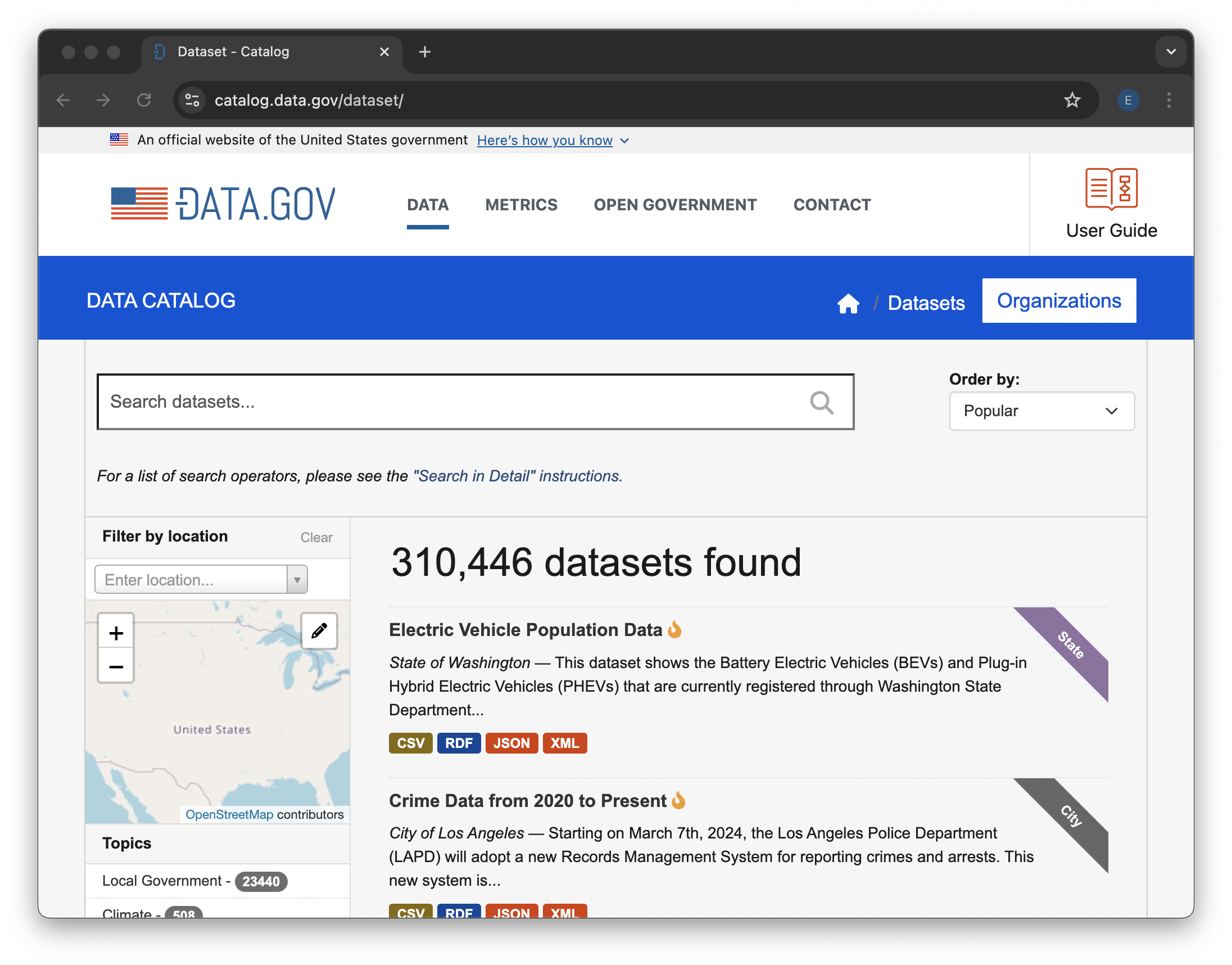
STEP 1A: Open up the data catalog

Click this link: https://catalog.data.gov. You can also open your web browser and type it in if you prefer.

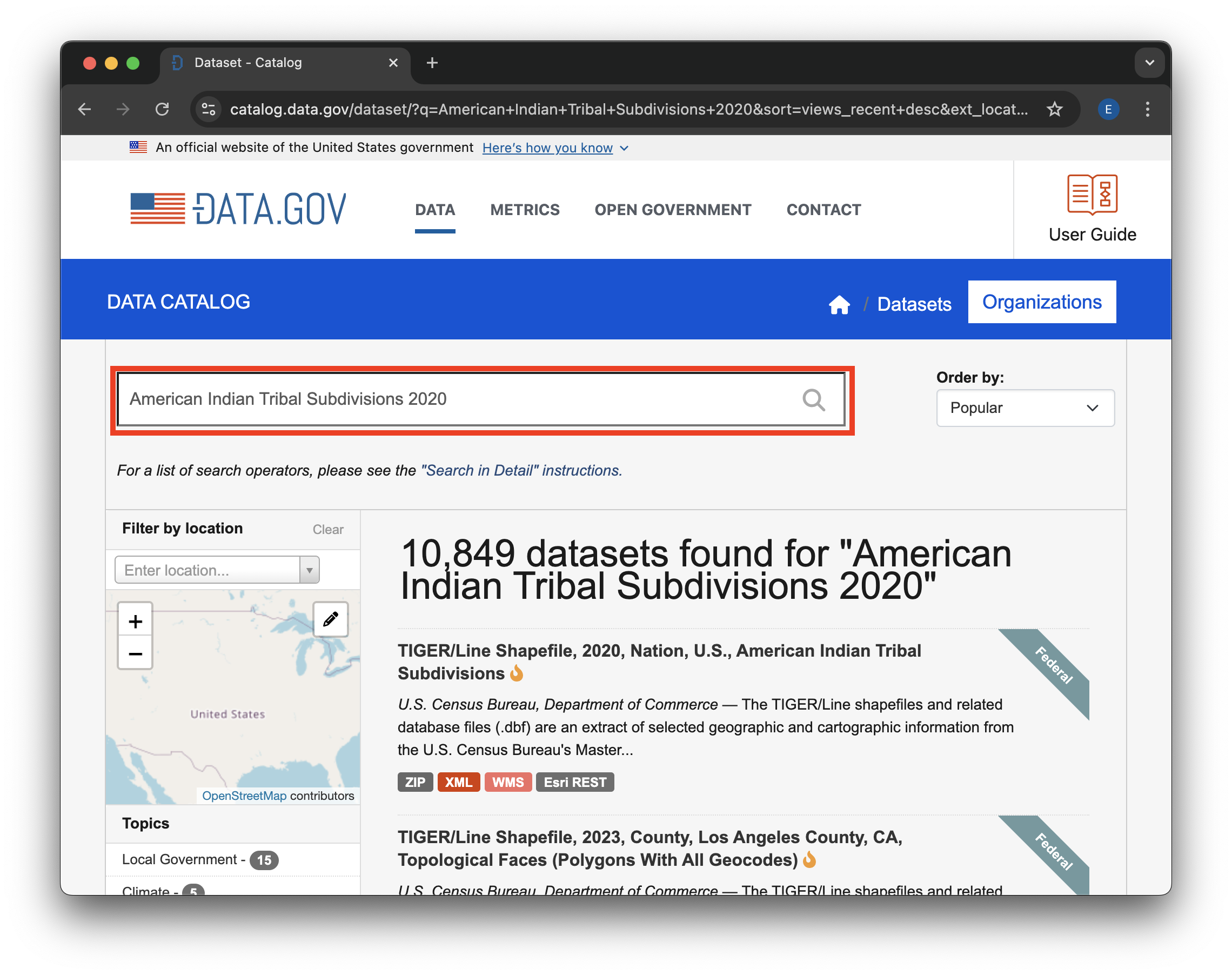
STEP 1B: Search

Search for the data you want. To get the American Indian Tribal Subdivisions census data, we recommend the search term “American Indian Tribal Subdivisions 2020”. These census files are updated regularly at the time of the census, so we want to make sure we have the most recent version. The last census was in 2020.

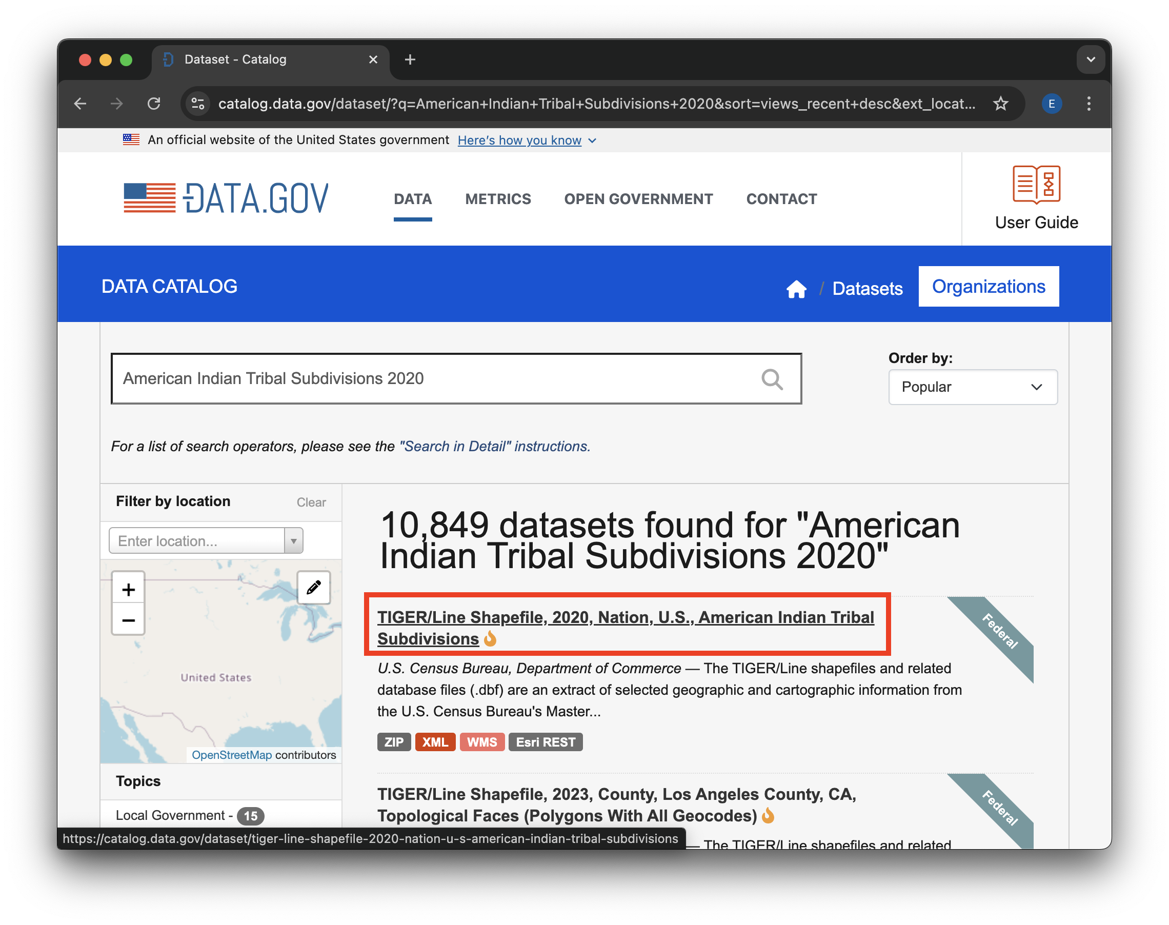
**Search** for “American Indian Tribal Subdivisions 2020”

STEP 1C: Open the dataset page

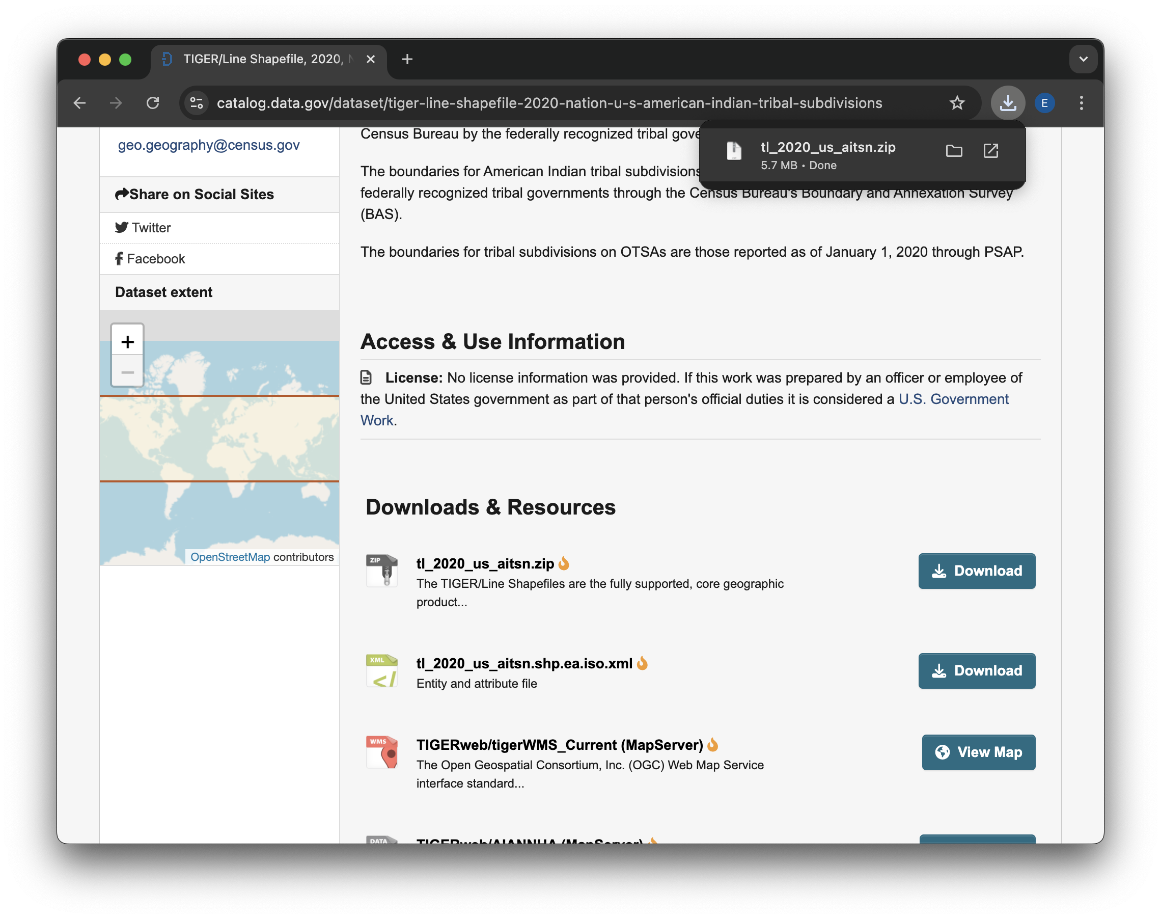
Find the “TIGER/Line Shapefile, 2020, Nation, U.S., American Indian Tribal Subdivisions” dataset in the search results, and click on the title to go to the dataset page.

Select the “TIGER/Line Shapefile, 2020, Nation, U.S., American Indian Tribal Subdivisions” dataset.

You should now be on the dataset page. ## STEP 1D: Download

Next, scroll down to the available files to download. Click on the Download button for the .zip file – this will be the easiest one to open in Python.

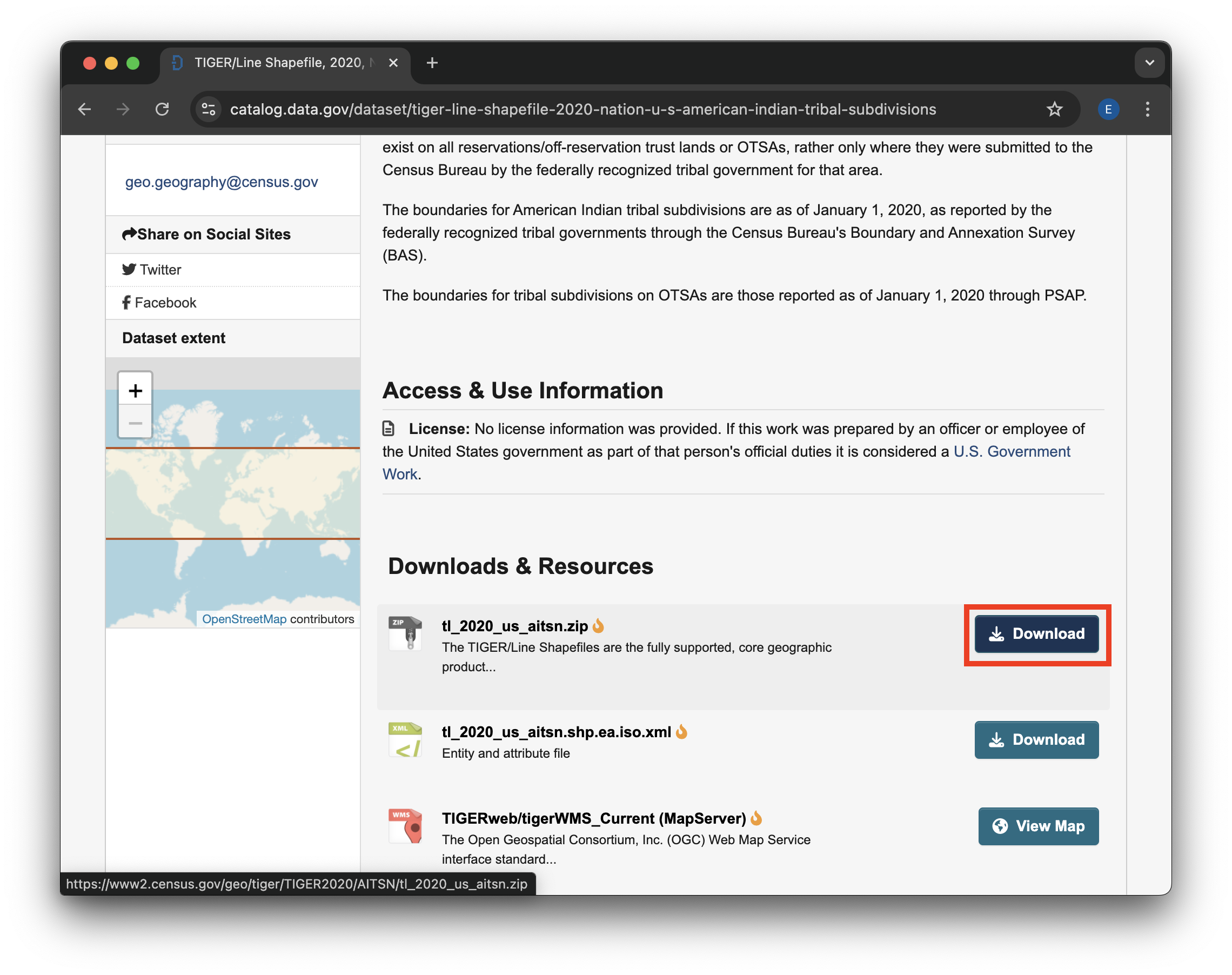
Scroll down and click on the `.zip` file `Download` button.

STEP 1E: Move your file

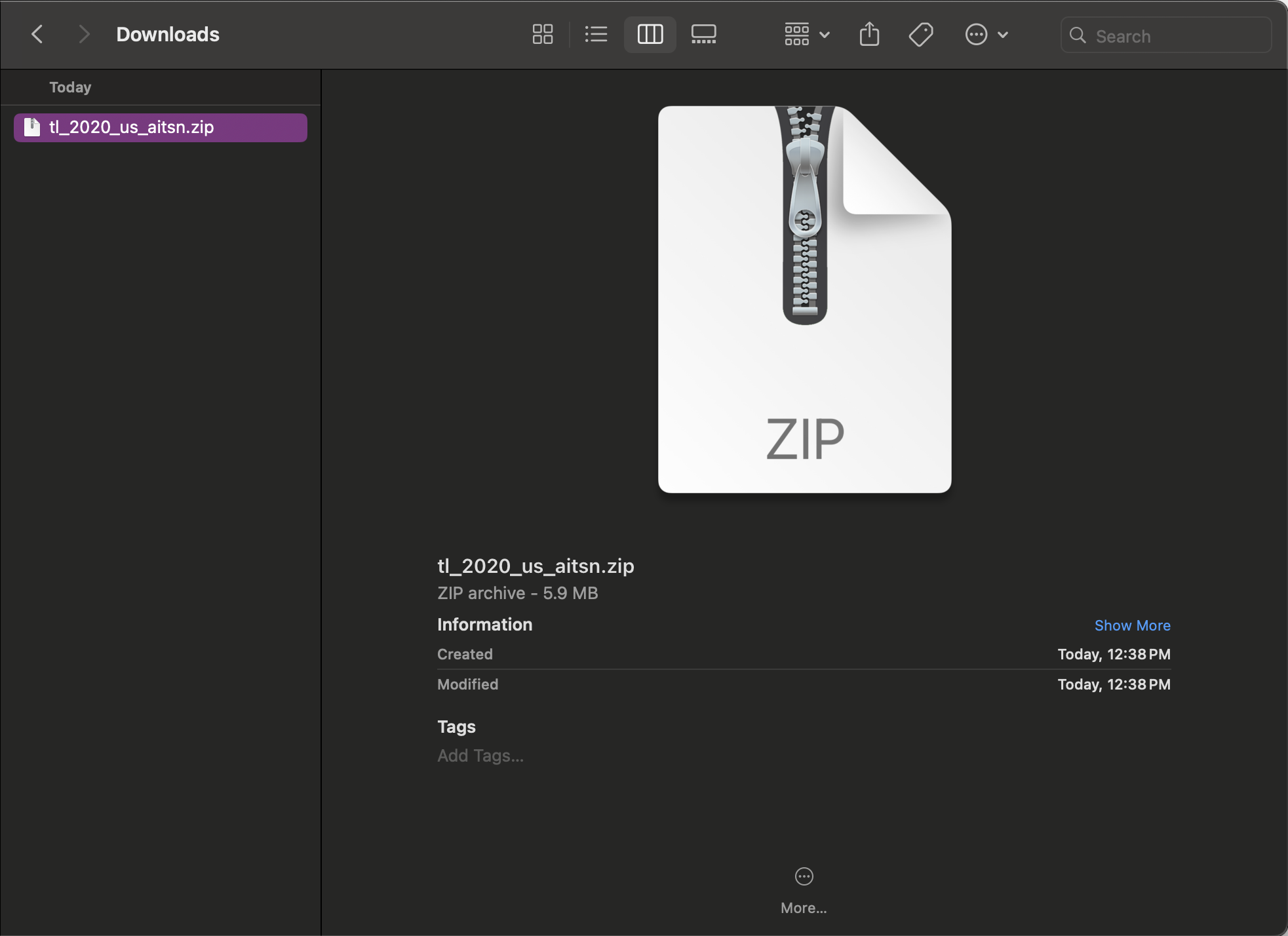
We now need to locate the file you downloaded and put it somewhere where Python can find it. Ideally, you should put the downloaded .zip file in your project directory. Most web browsers will pop up with some kind of button to open up your File Explorer (Windows) or Finder (Mac) in the location of your downloaded files. You can also check in your user home directory for a Downloads folder. If none of that works, try opening up your File Explorer/Finder and searching for the file

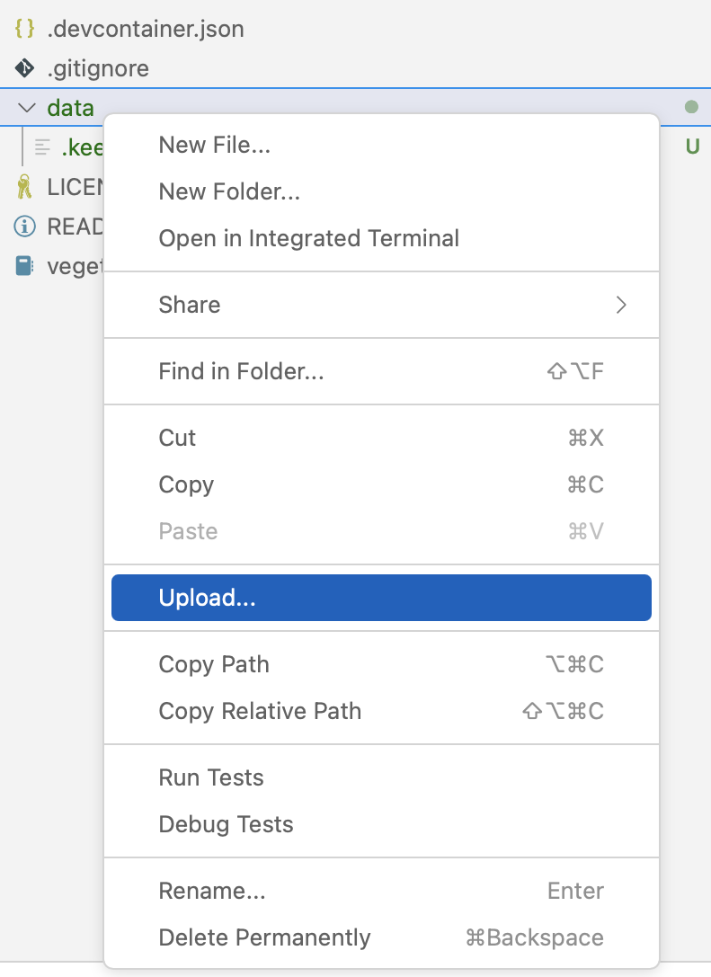
Open up the downloaded file in your Finder/File Explorer You should now see the file in your File Explorer/Finder

If you are working on GitHub Codespaces, you will need to upload your file before relocating it:

Go to the Explorer tab in your Codespace
Right-click on the data folder
Click Upload
Select the .zip file you just downloaded.

If you are using GitHub Codespaces, upload the file.

If you are working in GitHub Codespaces, you can skip ahead to unzipping the file! If not, you’ll need to relocate your file on your computer. One way to do that is with bash.

Try It

The code cell below is using a language called bash, which can be used to move files around your computer. To do that, we’re using the cp command, which stands for copy. In bash, you indicate that you want to retrieve a variable with the $ character. Since we’re in a Jupyter notebook, we can also access Python variables this way!

Check that the path to your file, ~/Downloads/tl_2020_us_aitsn.zip is accurate, and change it if it isn’t
Run the cell to move your file.

!cp ~/Downloads/tl_2020_us_aitsn.zip -d "$project.project_dir"

cp: cannot stat '/home/runner/Downloads/tl_2020_us_aitsn.zip': No such file or directory

Now, let’s check that the file got moved.

!ls "$project.project_dir"

tl_2020_us_aitsn.zip

You can optionally unzip the file. geopandas will be able to read this particular shapefile from a .zip archive, but some other files may need to be unzipped. We’ll first define the path in Python, and then use bash to unzip. You can also unzip with the Python zipfile library, but it is more complicated than we need right now.

filename = "tl_2020_us_aitsn"
zip_path = project.project_dir / f"{filename}.zip"
unzip_dir = project.project_dir / filename

The following command unzips a zip archive to the specified directory (-d). Any files that already exist are skipped without prompting (-n)

!unzip -n "$zip_path" -d "$unzip_dir"

Archive:  /home/runner/.local/share/earth-analytics/gila-river/tl_2020_us_aitsn.zip
 extracting: /home/runner/.local/share/earth-analytics/gila-river/tl_2020_us_aitsn/tl_2020_us_aitsn.cpg  
  inflating: /home/runner/.local/share/earth-analytics/gila-river/tl_2020_us_aitsn/tl_2020_us_aitsn.dbf  
  inflating: /home/runner/.local/share/earth-analytics/gila-river/tl_2020_us_aitsn/tl_2020_us_aitsn.prj  
  inflating: /home/runner/.local/share/earth-analytics/gila-river/tl_2020_us_aitsn/tl_2020_us_aitsn.shp  
  inflating: /home/runner/.local/share/earth-analytics/gila-river/tl_2020_us_aitsn/tl_2020_us_aitsn.shp.ea.iso.xml  
  inflating: /home/runner/.local/share/earth-analytics/gila-river/tl_2020_us_aitsn/tl_2020_us_aitsn.shp.iso.xml  
  inflating: /home/runner/.local/share/earth-analytics/gila-river/tl_2020_us_aitsn/tl_2020_us_aitsn.shx

You can also delete the zip file, now that it is extracted. This will help keep your data directory tidy:

!rm "$zip_path"

STEP 1F: Open boundary in Python

Try It

Replace "directory-name" with the actual name of the file you downloaded (or the folder you unzipped to) and put in your project directory.
Modify the code below to use descriptive variable names. Feel free to refer back to previous challenges for similar code!
Add a line of code to open up the data path. What library and function do you need to open this type of data?
Add some code to check your data, either by viewing it or making a quick plot. Does it look like what you expected?

# Define boundary path
path = project.project_dir / "directory-name"

# Open the site boundary


# Check that the data were downloaded correctly

See our solution!

# Define boundary path
aitsn_path = project.project_dir / "tl_2020_us_aitsn"

# Open the site boundary
aitsn_gdf = gpd.read_file(aitsn_path)

# Check that the data were downloaded correctly
aitsn_gdf.NAME

0                           Red Valley
1                           Rock Point
2                           Rough Rock
3                         Indian Wells
4                              Kayenta
                    ...               
479                                  1
480                  Mission Highlands
481                      Fort Thompson
482                       Indian Point
483    Cheyenne and Arapaho District 2
Name: NAME, Length: 484, dtype: object

Let’s go ahead and select the Gila River subdivisions, and make a site map.

Try It

Replace identifier with the value you found from exploring the interactive map. Make sure that you are using the correct data type!
Change the plot to have a web tile basemap, and look the way you want it to.

# Select and merge the subdivisions you want

# Plot the results with web tile images

See our solution!

# Select and merge the subdivisions you want
boundary_gdf = aitsn_gdf.loc[aitsn_gdf.AIANNHCE=='1310'].dissolve()
# Plot the results with web tile images
boundary_gdf.hvplot(
    geo=True, tiles='EsriImagery',
    fill_color=None, line_color='black',
    title=site_name,
    frame_width=500)

STEP 2: AppEEARS API

Exploring the AppEEARS API for NASA Earthdata access

Before you get started with the data download today, you will need a free NASA Earthdata account if you don’t have one already!

Over the next four cells, you will download MODIS NDVI data for the study period. MODIS is a multispectral instrument that measures Red and NIR data (and so can be used for NDVI). There are two MODIS sensors on two different platforms: satellites Terra and Aqua.

Learn more about MODIS datasets and the science they support

Since we’re asking for a special download that only covers our study area, we can’t just find a link to the data - we have to negotiate with the data server. We’re doing this using the APPEEARS API (Application Programming Interface). The API makes it possible for you to request data using code. You can use code from the earthpy library to handle the API request.

Try It

Often when we want to do something more complex in coding we find an example and modify it. This download code is already almost a working example. Your task will be:

Replace the start and end dates in the task parameters. Download data from July, when greenery is at its peak in the Northern Hemisphere.
Replace the year range. You should get 3 years before and after the event so you can see the change!
Replace gdf with the name of your site geodataframe.
Enter your NASA Earthdata username and password when prompted. The prompts can be a little hard to see – look at the top of your screen!

Reflect and Respond

What would the product and layer name be if you were trying to download Landsat Surface Temperature Analysis Ready Data (ARD) instead of MODIS NDVI?

Important

It can take some time for Appeears to process your request - anything from a few minutes to a few hours depending on how busy they are. You can check your progress by:

Going to the Appeears webpage
Clicking the Explore tab
Logging in with your Earthdata account

# Initialize AppeearsDownloader for MODIS NDVI data
ndvi_downloader = eaapp.AppeearsDownloader(
    download_key=download_key,
    ea_dir=project.project_dir,
    product='MOD13Q1.061',
    layer='_250m_16_days_NDVI',
    start_date="01-01",
    end_date="01-31",
    recurring=True,
    year_range=[2021, 2021],
    polygon=gdf
)
# Download the prepared download -- this can take some time!
ndvi_downloader.download_files(cache=True)

See our solution!

# Initialize AppeearsDownloader for MODIS NDVI data
ndvi_downloader = eaapp.AppeearsDownloader(
    download_key=download_key,
    project=project,
    product='MOD13Q1.061',
    layer='_250m_16_days_NDVI',
    start_date="06-01",
    end_date="09-01",
    recurring=True,
    year_range=[2001, 2007],
    polygon=boundary_gdf
)
# Download the prepared download -- this can take some time!
ndvi_downloader.download_files(cache=True)

<generator object Path.rglob at 0x7f6256a30ae0>

Putting it together: Working with multi-file raster datasets in Python

Now you need to load all the downloaded files into Python. You may have noticed that the `earthpy.appears module gives us all the downloaded file names…but only some of those are the NDVI files we want while others are quality files that tell us about the confidence in the dataset. For now, the files we want all have “NDVI” in the name.

Let’s start by getting all the NDVI file names. You will also need to extract the date from the filename. Check out the lesson on getting information from filenames in the textbook.

GOTCHA ALERT!

glob doesn’t necessarily find files in the order you would expect. Make sure to sort your file names like it says in the textbook.

# Get a list of NDVI tif file paths

See our solution!

# Get list of NDVI tif file paths
ndvi_paths = sorted(glob(os.path.join(
    project.project_dir, '**', '*NDVI*.tif')))
f'{len(ndvi_paths)} NDVI paths found'

'0 NDVI paths found'

Repeating tasks in Python

Now you should have a few dozen files! For each file, you need to:

Load the file in using the rioxarray library
Get the date from the file name
Add the date as a dimension coordinate
Give your data variable a name

You don’t want to write out the code for each file! That’s a recipe for copy pasta and errors. Luckily, Python has tools for doing similar tasks repeatedly. In this case, you’ll use one called a for loop.

There’s some code below that uses a for loop in what is called an accumulation pattern to process each file. That means that you will save the results of your processing to a list each time you process the files, and then merge all the arrays in the list.

Try It

Look at the file names. How many characters from the end is the date? doy_start and doy_end are used to extract the day of the year (doy) from the file name. You will need to count characters from the end and change the values to get the right part of the file name. HINT: the index -1 in Python means the last value, -2 second-to-last, and so on.
Replace any required variable names with your chosen variable names

doy_start = -1
doy_end = -1

# Loop through each NDVI image
ndvi_das = []
for ndvi_path in ndvi_paths:
    # Get date from file name

    # Open dataset

    # Add date dimension and clean up metadata
    da = da.assign_coords({'date': date})
    da = da.expand_dims({'date': 1})
    da.name = 'NDVI'

    # Prepare for concatenation

See our solution!

doy_start = -19
doy_end = -12

# Loop through each NDVI image
ndvi_das = []
for ndvi_path in ndvi_paths:
    # Get date from file name
    doy = ndvi_path[doy_start:doy_end]
    date = pd.to_datetime(doy, format='%Y%j')

    # Open dataset
    da = rxr.open_rasterio(ndvi_path, mask_and_scale=True).squeeze()

    # Add date dimension and clean up metadata
    da = da.assign_coords({'date': date})
    da = da.expand_dims({'date': 1})
    da.name = 'NDVI'

    # Prepare for concatenation
    ndvi_das.append(da)

len(ndvi_das)

Try It

Next, stack your arrays by date into a time series:

Modify the code to match your prior workflow steps and to use descriptive variable names
Replace coordinate_name with the actual name of the coordinate you want to build up.

# Combine NDVI images from all dates
da = xr.combine_by_coords(list_of_data_arrays, coords=['coordinate_name'])
da

See our solution!

# Combine NDVI images from all dates
ndvi_da = xr.combine_by_coords(ndvi_das, coords=['date'])
ndvi_da

<xarray.Dataset> Size: 0B
Dimensions:  ()
Data variables:
    *empty*

Your turn! Repeat this workflow in a different time and place.

It’s not only irrigation that affects NDVI! You could look at:

Recovery after a national disaster, like a wildfire or hurricane
Drought
Deforestation
Irrigation
Beaver reintroduction