Water Rights Restored to the Gila River

The impacts of irrigation on vegetation health in the Gila River Valley

In 2004, the Akimel O’‘otham and Tohono O’’odham tribes won a water rights settlement in the US Supreme Court. Using satellite imagery, we can see the effects of irrigation water on the local vegetation.

Learning Goals:

• Open raster or image data using code
• Combine raster data and vector data to crop images to an area of interest
• Summarize raster values with stastics
• Analyze a time-series of raster images

Reclaiming Water Rights on the Gila River

The Gila River Reservation south of Phoenix, AZ is the ancestral home of the Akimel O’otham and Tohono O’odham tribes. The Gila River area was known for its agriculture, with miles of canals providing irrigation. However, in the 1800s, European colonizers upstream installed dams which cut off water supply. This resulted in the collapse of Gila River agriculture, along with sky-rocketing rates of diabetes and heart disease in the community as they were force to subsist only on US government surplus rations.

In 2004, the Gila River community won back much of its water rights in court. The settlement granted senior water rights nearly matching pre-colonial water use. Work has begun to rebuild the agriculture in the Gila River Reservation. According to the Akimel O’otham and Tohono O’odham tribes, “It will take years to complete but in the end the community members will once again hear the sweet music of rushing water.”

Observing vegetation health from space

We will look at vegetation health using NDVI (Normalized Difference Vegetation Index). How does it work? First, we need to learn about spectral reflectance signatures.

Every object reflects some wavelengths of light more or less than others. We can see this with our eyes, since, for example, plants reflect a lot of green in the summer, and then as that green diminishes in the fall they look more yellow or orange. The image below shows spectral signatures for water, soil, and vegetation:

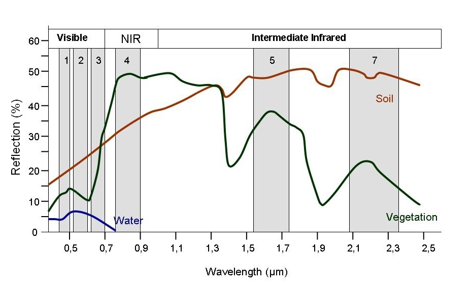> Image source: SEOS Project

Healthy vegetation reflects a lot of Near-InfraRed (NIR) radiation. Less healthy vegetation reflects a similar amounts of the visible light spectra, but less NIR radiation. We don’t see a huge drop in Green radiation until the plant is very stressed or dead. That means that NIR allows us to get ahead of what we can see with our eyes.

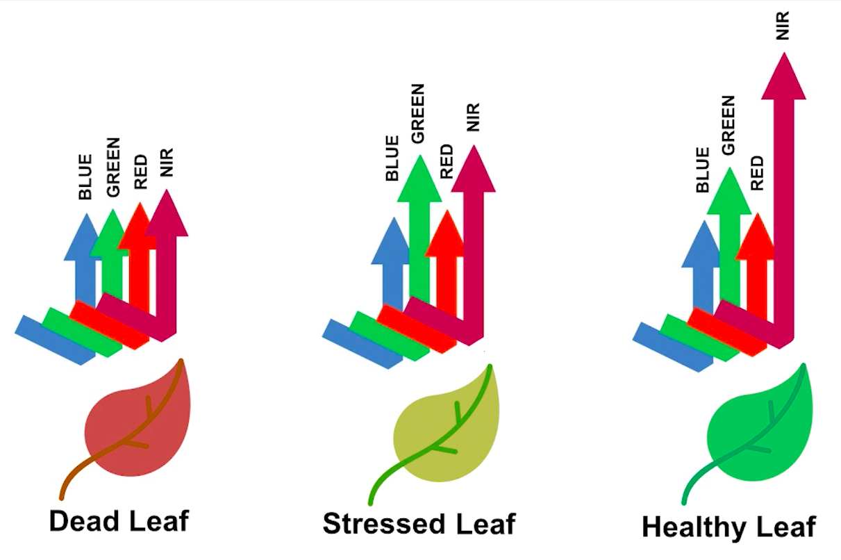> Image source: Spectral signature literature review by px39n

Different species of plants reflect different spectral signatures, but the pattern of the signatures across species and sitations is similar. NDVI compares the amount of NIR reflectance to the amount of Red reflectance, thus accounting for many of the species differences and isolating the health of the plant. The formula for calculating NDVI is:

\[NDVI = \frac{(NIR - Red)}{(NIR + Red)}\]

Read More

Read more about NDVI and other vegetation indices:

• earthdatascience.org
• USGS

Before we get started coding, you can use the following parameters to change things about the workflow:

id = 'stars'
site_name = 'Gila River Indian Community'
event = 'water rights case'
data_dir = 'gila-river'

STEP 1: Site map

We’ll need some Python libraries to complete this workflow.

Try It: Import necessary libraries

In the cell below, making sure to keep the packages in order, add packages for:

• Working with DataFrames
• Working with GeoDataFrames
• Making interactive plots of tabular and vector data

Reflect and Respond

What are we using the rest of these packages for? See if you can figure it out as you complete the notebook.

import json
import os
import pathlib

import hvplot.xarray
import rioxarray as rxr
import xarray as xr

import json
from glob import glob

import earthpy
import geopandas as gpd
import hvplot.pandas
import hvplot.xarray
import pandas as pd
import rioxarray as rxr
import xarray as xr

We have one more setup task. We’re not going to be able to load all our data directly from the web to Python this time. That means we need to set up a place for it.

GOTCHA ALERT!

A lot of times in Python we say “directory” to mean a “folder” on your computer. The two words mean the same thing in this context.

Try It

In the cell below, replace ‘my-data-folder’ with a descriptive directory name.

project = earthpy.Project("Gila River Vegetation", dirname='my-data-folder')
project.get_data()

project = earthpy.Project("Gila River Vegetation")
project.get_data()

**Final Configuration Loaded:**
{}
🔄 Fetching metadata for article 29170118...
✅ Found 2 files for download.
[('https://ndownloader.figshare.com/files/54896597', 'gila-river-ndvi', 'zip'), ('https://ndownloader.figshare.com/files/54896600', 'tl_2020_us_aitsn', 'zip')]
gila-river-ndvi
Downloading from https://ndownloader.figshare.com/files/54896597
Extracted output to /home/runner/.local/share/earth-analytics/gila-river-vegetation/gila-river-ndvi
[PosixPath('/home/runner/.local/share/earth-analytics/gila-river-vegetation/gila-river-ndvi')]
tl_2020_us_aitsn
Downloading from https://ndownloader.figshare.com/files/54896600
Extracted output to /home/runner/.local/share/earth-analytics/gila-river-vegetation/tl_2020_us_aitsn
[PosixPath('/home/runner/.local/share/earth-analytics/gila-river-vegetation/gila-river-ndvi'), PosixPath('/home/runner/.local/share/earth-analytics/gila-river-vegetation/tl_2020_us_aitsn')]

Study Area: Gila River Indian Community

Earth Data Science data formats

In Earth Data Science, we get data in three main formats:

Data type	Descriptions	Common file formats	Python type
Time Series	The same data points (e.g. streamflow) collected multiple times over time	Tabular formats (e.g. .csv, or .xlsx)	pandas DataFrame
Vector	Points, lines, and areas (with coordinates)	Shapefile (often an archive like a .zip file because a Shapefile is actually a collection of at least 3 files)	geopandas GeoDataFrame
Raster	Evenly spaced spatial grid (with coordinates)	GeoTIFF (.tif), NetCDF (.nc), HDF (.hdf)	rioxarray DataArray

Read More

Check out the sections about about vector data and raster data in the textbook.

Reflect and Respond

For this coding challenge, we are interested in the boundary of the Gila River Indian Community, and the health of vegetation in the area measured on a scale from -1 to 1. In the cell below, answer the following question: What data type do you think the boundary will be? What about the vegetation health?

Load the Gila River Indian Community boundary

Try It

• Locate the Tribal Subdivision files in your download directory
• Change 'subdivision-directory' to the actual location
• Load the data into Python and check that it worked

# Load in the boundary data
aitsn_gdf = gpd.read_file(project.project_dir / 'subdivision-directory')
# Check that it worked

# Load in the boundary data
aitsn_gdf = gpd.read_file(project.project_dir / 'tl_2020_us_aitsn')
# Check that it worked
aitsn_gdf

	AIANNHCE	TRSUBCE	TRSUBNS	GEOID	NAME	NAMELSAD	LSAD	CLASSFP	MTFCC	FUNCSTAT	ALAND	AWATER	INTPTLAT	INTPTLON	geometry
0	2430	653	02419073	2430653	Red Valley	Red Valley Chapter	T2	D7	G2300	A	922036695	195247	+36.6294607	-109.0550394	POLYGON ((-109.2827 36.64644, -109.28181 36.65...
1	2430	665	02419077	2430665	Rock Point	Rock Point Chapter	T2	D7	G2300	A	720360268	88806	+36.6598701	-109.6166836	POLYGON ((-109.85922 36.49859, -109.85521 36.5...
2	2430	675	02419081	2430675	Rough Rock	Rough Rock Chapter	T2	D7	G2300	A	364475668	216144	+36.3976971	-109.7695183	POLYGON ((-109.93053 36.40672, -109.92923 36.4...
3	2430	325	02418975	2430325	Indian Wells	Indian Wells Chapter	T2	D7	G2300	A	717835323	133795	+35.3248534	-110.0855000	POLYGON ((-110.24222 35.36327, -110.24215 35.3...
4	2430	355	02418983	2430355	Kayenta	Kayenta Chapter	T2	D7	G2300	A	1419241065	1982848	+36.6884391	-110.3045616	POLYGON ((-110.56817 36.73489, -110.56603 36.7...
...	...	...	...	...	...	...	...	...	...	...	...	...	...	...	...
479	1310	100	02418907	1310100	1	District 1	28	D7	G2300	N	139902197	0	+33.0600842	-111.5806313	POLYGON ((-111.63622 33.11798, -111.63405 33.1...
480	4290	550	02612186	4290550	Mission Highlands	Mission Highlands	00	D7	G2300	N	6188043	0	+48.0754384	-122.2507432	POLYGON ((-122.27579 48.07128, -122.27578 48.0...
481	0855	400	02418941	0855400	Fort Thompson	Fort Thompson District	07	D7	G2300	N	535432708	38653364	+44.1559680	-099.4467700	POLYGON ((-99.66452 44.25269, -99.66449 44.255...
482	0335	300	02784108	0335300	Indian Point	Indian Point Segment	T3	D7	G2300	N	326985	0	+48.0604594	-092.8466753	POLYGON ((-92.85187 48.05944, -92.85186 48.059...
483	5560	120	02804808	5560120	Cheyenne and Arapaho District 2	Cheyenne and Arapaho District 2	00	D7	G2300	S	4709525489	36177523	+35.7613633	-098.0107463	POLYGON ((-98.61081 35.72524, -98.60732 35.725...

484 rows × 15 columns

You might notice in this dataset that some of the names are not easily searchable. For example, the Gila River subdivisions are named “District 1-7”! So, how do we know what to search for? We recommend making an interactive plot of the data so that you can find the information you need, e.g.:

aitsn_gdf.hvplot(
    geo=True, tiles='EsriImagery', 
    frame_width=500,
    legend=False, fill_color=None, edge_color='white',
    # This parameter makes all the column values in the dataset visible.
    hover_cols='all')

WARNING:param.main: edge_color option not found for polygons plot with bokeh; similar options include: ['muted_color', 'bgcolor', 'line_color']

Reflect and Respond

What column could you use to uniquely identify the subdivisions of the reservation you want to study using this interactive map? What value do you need to use to filter the GeoDataFrame?

Now that you have the info you need, it’s also a good idea to check the data type. For example, we suggest looking at the AIANNHCE column…but is that value some kind of number or an object like a text string? We can’t tell just by looking, which is where our friend the .info() method comes in:

aitsn_gdf.info()

<class 'geopandas.geodataframe.GeoDataFrame'>
RangeIndex: 484 entries, 0 to 483
Data columns (total 15 columns):
 #   Column    Non-Null Count  Dtype   
---  ------    --------------  -----   
 0   AIANNHCE  484 non-null    object  
 1   TRSUBCE   484 non-null    object  
 2   TRSUBNS   484 non-null    object  
 3   GEOID     484 non-null    object  
 4   NAME      484 non-null    object  
 5   NAMELSAD  484 non-null    object  
 6   LSAD      484 non-null    object  
 7   CLASSFP   484 non-null    object  
 8   MTFCC     484 non-null    object  
 9   FUNCSTAT  484 non-null    object  
 10  ALAND     484 non-null    int64   
 11  AWATER    484 non-null    int64   
 12  INTPTLAT  484 non-null    object  
 13  INTPTLON  484 non-null    object  
 14  geometry  484 non-null    geometry
dtypes: geometry(1), int64(2), object(12)
memory usage: 56.8+ KB

Reflect and Respond

What is the data type of the AIANNHCE column? How will that affect your code?

Let’s go ahead and select the Gila River subdivisions, and make a site map.

Try It

1. Replace identifier with the value you found from exploring the interactive map. Make sure that you are using the correct data type!
2. Change the plot to have a web tile basemap, and look the way you want it to.

# Select and merge the subdivisions you want
gdf = aitsn_gdf.loc[aitsn_gdf.AIANNHCE==identifier].dissolve()
# Plot the results with web tile images
gdf.hvplot()

# Select and merge the subdivisions you want
boundary_gdf = aitsn_gdf.loc[aitsn_gdf.AIANNHCE=='1310'].dissolve()
# Plot the results with web tile images
boundary_gdf.hvplot(
    geo=True, tiles='EsriImagery',
    fill_color=None, line_color='black',
    title=site_name,
    frame_width=500)

STEP 2: Wrangle Raster Data

Load in NDVI data

Now you need to load all the downloaded files into Python. Let’s start by getting all the file names. You will also need to extract the date from the filename. Check out the lesson on getting information from filenames in the textbook.

In this lesson, you will use the glob.glob() function in Python to find all files that match a pattern formed with the wildcard character *. The wildcard can represent any string of alphanumberic characters. For example, the pattern 'file_*.tif' will match the files 'file_1.tif', 'file_2.tiv', or even 'file_qeoiurghtfoqaegbn34pf.tif'… but it will not match 'something-else.csv' or even 'something-else.tif'.

In this notebook, we’ll use the .rglob(), or recursive glob method of the Path object instead. It works similarly, but you’ll notice that we have to convert the results to a list with the list() function.

GOTCHA ALERT!

glob doesn’t necessarily find files in the order you would expect. Make sure to sort your file names like it says in the textbook.

Reflect and Respond

Take a look at the file names for the NDVI files. What do you notice is the same for all the files? Keep in mind that you only want the NDVI files, not the Quality files (which will flag potential incorrect measurements).

Try It

1. Create a pattern for the files you want to import. Your pattern should include the parts of the file names that are the same for all files, and replace the rest with the * character. Make sure to match the NDVI files, but not the Quality files!
2. Replace ndvi-pattern with your pattern
3. Run the code and make sure that you are getting all the files you want and none of the files you don’t!

# Get a sorted list of NDVI tif file paths
ndvi_paths = sorted(list(project.project_dir.rglob('ndvi-pattern')))

# Display the first and last three files paths to check the pattern
ndvi_paths[:3], ndvi_paths[-3:]

# Get a sorted list of NDVI tif file paths
ndvi_paths = sorted(list(project.project_dir.rglob('*NDVI*.tif')))

# Display the first and last three files paths to check the pattern
ndvi_paths[:3], ndvi_paths[-3:]

([PosixPath('/home/runner/.local/share/earth-analytics/gila-river-vegetation/gila-river-ndvi/MOD13Q1.061_2001137_to_2007244/MOD13Q1.061__250m_16_days_NDVI_doy2001145_aid0001.tif'),
  PosixPath('/home/runner/.local/share/earth-analytics/gila-river-vegetation/gila-river-ndvi/MOD13Q1.061_2001137_to_2007244/MOD13Q1.061__250m_16_days_NDVI_doy2001161_aid0001.tif'),
  PosixPath('/home/runner/.local/share/earth-analytics/gila-river-vegetation/gila-river-ndvi/MOD13Q1.061_2001137_to_2007244/MOD13Q1.061__250m_16_days_NDVI_doy2001177_aid0001.tif')],
 [PosixPath('/home/runner/.local/share/earth-analytics/gila-river-vegetation/gila-river-ndvi/MOD13Q1.061_2001137_to_2007244/MOD13Q1.061__250m_16_days_NDVI_doy2007209_aid0001.tif'),
  PosixPath('/home/runner/.local/share/earth-analytics/gila-river-vegetation/gila-river-ndvi/MOD13Q1.061_2001137_to_2007244/MOD13Q1.061__250m_16_days_NDVI_doy2007225_aid0001.tif'),
  PosixPath('/home/runner/.local/share/earth-analytics/gila-river-vegetation/gila-river-ndvi/MOD13Q1.061_2001137_to_2007244/MOD13Q1.061__250m_16_days_NDVI_doy2007241_aid0001.tif')])

Repeating tasks in Python

Now you should have a few dozen files! For each file, you need to:

• Load the file in using the rioxarray library
• Get the date from the file name
• Add the date as a dimension coordinate
• Give your data variable a name

You don’t want to write out the code for each file! That’s a recipe for copy pasta. Luckily, Python has tools for doing similar tasks repeatedly. In this case, you’ll use one called a for loop.

There’s some code below that uses a for loop in what is called an accumulation pattern to process each file. That means that you will save the results of your processing to a list each time you process the files, and then merge all the arrays in the list.

Try It

• Look at the file names. How many characters from the end is the date? doy_start and doy_end are used to extract the day of the year (doy) from the file name. You will need to count characters from the end and change the values to get the right part of the file name. HINT: the index -1 in Python means the last value, -2 second-to-last, and so on.
• Replace any required variable names with your chosen variable names

doy_start = -1
doy_end = -1

# Loop through each NDVI image
ndvi_das = []
for ndvi_path in ndvi_paths:
    # Get date from file name

    # Open dataset

    # Add date dimension and clean up metadata
    da = da.assign_coords({'date': date})
    da = da.expand_dims({'date': 1})
    da.name = 'NDVI'

    # Prepare for concatenation

doy_start = -19
doy_end = -12

# Loop through each NDVI image
ndvi_das = []
for ndvi_path in ndvi_paths:
    # Get date from the file name
    doy = ndvi_path.name[doy_start:doy_end]
    date = pd.to_datetime(doy, format='%Y%j')

    # Open dataset
    da = rxr.open_rasterio(ndvi_path, mask_and_scale=True).squeeze()

    # Add date dimension and clean up metadata
    da = da.assign_coords({'date': date})
    da = da.expand_dims({'date': 1})
    da.name = 'NDVI'

    # Prepare for concatenation
    ndvi_das.append(da)

len(ndvi_das)

49

Combine Rasters

Next, stack your arrays by date into a time series using the xr.combine_by_coords() function. You will have to tell it which dimension you want to stack your data in.

# Combine NDVI images from all dates

# Combine NDVI images from all dates
ndvi_da = xr.combine_by_coords(ndvi_das, coords=['date'])
ndvi_da

<xarray.Dataset> Size: 15MB
Dimensions:      (date: 49, y: 203, x: 382)
Coordinates:
    band         int64 8B 1
  * x            (x) float64 3kB -112.3 -112.3 -112.3 ... -111.5 -111.5 -111.5
  * y            (y) float64 2kB 33.39 33.39 33.38 33.38 ... 32.97 32.97 32.97
    spatial_ref  int64 8B 0
  * date         (date) datetime64[ns] 392B 2001-05-25 2001-06-10 ... 2007-08-29
Data variables:
    NDVI         (date, y, x) float32 15MB 0.8282 0.6146 ... 0.2712 0.2602

xarray.Dataset

• Dimensions:
  • date: 49
  • y: 203
  • x: 382
• Coordinates: (5)
  • band
    ()
    int64
    1

    array(1)

  • x
    (x)
    float64
    -112.3 -112.3 ... -111.5 -111.5

    array([-112.309375, -112.307292, -112.305208, ..., -111.519792, -111.517708,
           -111.515625], shape=(382,))

  • y
    (y)
    float64
    33.39 33.39 33.38 ... 32.97 32.97

    array([33.388542, 33.386458, 33.384375, ..., 32.971875, 32.969792, 32.967708],
          shape=(203,))

  • spatial_ref
    ()
    int64
    0

    crs_wkt :

    GEOGCS["WGS 84",DATUM["WGS_1984",SPHEROID["WGS 84",6378137,298.257223563,AUTHORITY["EPSG","7030"]],AUTHORITY["EPSG","6326"]],PRIMEM["Greenwich",0,AUTHORITY["EPSG","8901"]],UNIT["degree",0.0174532925199433,AUTHORITY["EPSG","9122"]],AXIS["Latitude",NORTH],AXIS["Longitude",EAST],AUTHORITY["EPSG","4326"]]

    semi_major_axis :

    6378137.0

    semi_minor_axis :

    6356752.314245179

    inverse_flattening :

    298.257223563

    reference_ellipsoid_name :

    WGS 84

    longitude_of_prime_meridian :

    0.0

    prime_meridian_name :

    Greenwich

    geographic_crs_name :

    WGS 84

    horizontal_datum_name :

    World Geodetic System 1984

    grid_mapping_name :

    latitude_longitude

    spatial_ref :

    GEOGCS["WGS 84",DATUM["WGS_1984",SPHEROID["WGS 84",6378137,298.257223563,AUTHORITY["EPSG","7030"]],AUTHORITY["EPSG","6326"]],PRIMEM["Greenwich",0,AUTHORITY["EPSG","8901"]],UNIT["degree",0.0174532925199433,AUTHORITY["EPSG","9122"]],AXIS["Latitude",NORTH],AXIS["Longitude",EAST],AUTHORITY["EPSG","4326"]]

    GeoTransform :

    -112.31041665660531 0.0020833333331466974 0.0 33.38958333034212 0.0 -0.0020833333331466974

    array(0)

  • date
    (date)
    datetime64[ns]
    2001-05-25 ... 2007-08-29

    array(['2001-05-25T00:00:00.000000000', '2001-06-10T00:00:00.000000000',
           '2001-06-26T00:00:00.000000000', '2001-07-12T00:00:00.000000000',
           '2001-07-28T00:00:00.000000000', '2001-08-13T00:00:00.000000000',
           '2001-08-29T00:00:00.000000000', '2002-05-25T00:00:00.000000000',
           '2002-06-10T00:00:00.000000000', '2002-06-26T00:00:00.000000000',
           '2002-07-12T00:00:00.000000000', '2002-07-28T00:00:00.000000000',
           '2002-08-13T00:00:00.000000000', '2002-08-29T00:00:00.000000000',
           '2003-05-25T00:00:00.000000000', '2003-06-10T00:00:00.000000000',
           '2003-06-26T00:00:00.000000000', '2003-07-12T00:00:00.000000000',
           '2003-07-28T00:00:00.000000000', '2003-08-13T00:00:00.000000000',
           '2003-08-29T00:00:00.000000000', '2004-05-24T00:00:00.000000000',
           '2004-06-09T00:00:00.000000000', '2004-06-25T00:00:00.000000000',
           '2004-07-11T00:00:00.000000000', '2004-07-27T00:00:00.000000000',
           '2004-08-12T00:00:00.000000000', '2004-08-28T00:00:00.000000000',
           '2005-05-25T00:00:00.000000000', '2005-06-10T00:00:00.000000000',
           '2005-06-26T00:00:00.000000000', '2005-07-12T00:00:00.000000000',
           '2005-07-28T00:00:00.000000000', '2005-08-13T00:00:00.000000000',
           '2005-08-29T00:00:00.000000000', '2006-05-25T00:00:00.000000000',
           '2006-06-10T00:00:00.000000000', '2006-06-26T00:00:00.000000000',
           '2006-07-12T00:00:00.000000000', '2006-07-28T00:00:00.000000000',
           '2006-08-13T00:00:00.000000000', '2006-08-29T00:00:00.000000000',
           '2007-05-25T00:00:00.000000000', '2007-06-10T00:00:00.000000000',
           '2007-06-26T00:00:00.000000000', '2007-07-12T00:00:00.000000000',
           '2007-07-28T00:00:00.000000000', '2007-08-13T00:00:00.000000000',
           '2007-08-29T00:00:00.000000000'], dtype='datetime64[ns]')

• Data variables: (1)
  • NDVI
    (date, y, x)
    float32
    0.8282 0.6146 ... 0.2712 0.2602

    units :

    NDVI

    AREA_OR_POINT :

    Area

    array([[[0.8282    , 0.6146    , 0.3796    , ..., 0.1542    ,
             0.1542    , 0.1774    ],
            [0.52349997, 0.32029998, 0.46359998, ..., 0.145     ,
             0.145     , 0.145     ],
            [0.52349997, 0.38509998, 0.4567    , ..., 0.0962    ,
             0.058     , 0.0641    ],
            ...,
            [0.13759999, 0.13759999, 0.1283    , ..., 0.1489    ,
             0.1489    , 0.1568    ],
            [0.1299    , 0.1299    , 0.12379999, ..., 0.1831    ,
             0.1831    , 0.23169999],
            [0.1347    , 0.1309    , 0.1329    , ..., 0.15709999,
             0.2384    , 0.2452    ]],
    
           [[0.5146    , 0.42249998, 0.3706    , ..., 0.1656    ,
             0.1656    , 0.1656    ],
            [0.3543    , 0.4138    , 0.3706    , ..., 0.1275    ,
             0.1275    , 0.0968    ],
            [0.48029998, 0.3543    , 0.3687    , ..., 0.075     ,
             0.075     , 0.0968    ],
    ...
            [0.14469999, 0.14469999, 0.12789999, ..., 0.17      ,
             0.17      , 0.15959999],
            [0.1382    , 0.1382    , 0.12969999, ..., 0.2052    ,
             0.2052    , 0.2259    ],
            [0.1407    , 0.126     , 0.1345    , ..., 0.23879999,
             0.2481    , 0.2883    ]],
    
           [[0.7557    , 0.7066    , 0.46179998, ..., 0.12789999,
             0.12789999, 0.1379    ],
            [0.57739997, 0.3434    , 0.46179998, ..., 0.12789999,
             0.12789999, 0.1187    ],
            [0.5342    , 0.4926    , 0.3505    , ..., 0.1054    ,
             0.1054    , 0.0465    ],
            ...,
            [0.1255    , 0.1255    , 0.1255    , ..., 0.17      ,
             0.17      , 0.1724    ],
            [0.1205    , 0.1205    , 0.1258    , ..., 0.22909999,
             0.22909999, 0.24      ],
            [0.1469    , 0.1284    , 0.1258    , ..., 0.19919999,
             0.2712    , 0.2602    ]]], shape=(49, 203, 382), dtype=float32)

• Indexes: (3)
  • x
    PandasIndex

    PandasIndex(Index([-112.30937498993873, -112.30729165660559, -112.30520832327244,
           -112.30312498993929, -112.30104165660615,   -112.298958323273,
           -112.29687498993985,  -112.2947916566067, -112.29270832327356,
           -112.29062498994041,
           ...
           -111.53437499000816, -111.53229165667501, -111.53020832334187,
           -111.52812499000872, -111.52604165667557, -111.52395832334243,
           -111.52187499000928, -111.51979165667613, -111.51770832334299,
           -111.51562499000984],
          dtype='float64', name='x', length=382))

  • y
    PandasIndex

    PandasIndex(Index([ 33.38854166367555,   33.3864583303424,  33.38437499700925,
            33.38229166367611,  33.38020833034296,  33.37812499700981,
           33.376041663676666,  33.37395833034352,  33.37187499701037,
           33.369791663677226,
           ...
           32.986458330378234,  32.98437499704509,  32.98229166371194,
           32.980208330378794,  32.97812499704565,   32.9760416637125,
           32.973958330379354,  32.97187499704621,  32.96979166371306,
           32.967708330379914],
          dtype='float64', name='y', length=203))

  • date
    PandasIndex

    PandasIndex(DatetimeIndex(['2001-05-25', '2001-06-10', '2001-06-26', '2001-07-12',
                   '2001-07-28', '2001-08-13', '2001-08-29', '2002-05-25',
                   '2002-06-10', '2002-06-26', '2002-07-12', '2002-07-28',
                   '2002-08-13', '2002-08-29', '2003-05-25', '2003-06-10',
                   '2003-06-26', '2003-07-12', '2003-07-28', '2003-08-13',
                   '2003-08-29', '2004-05-24', '2004-06-09', '2004-06-25',
                   '2004-07-11', '2004-07-27', '2004-08-12', '2004-08-28',
                   '2005-05-25', '2005-06-10', '2005-06-26', '2005-07-12',
                   '2005-07-28', '2005-08-13', '2005-08-29', '2006-05-25',
                   '2006-06-10', '2006-06-26', '2006-07-12', '2006-07-28',
                   '2006-08-13', '2006-08-29', '2007-05-25', '2007-06-10',
                   '2007-06-26', '2007-07-12', '2007-07-28', '2007-08-13',
                   '2007-08-29'],
                  dtype='datetime64[ns]', name='date', freq=None))

• Attributes: (0)

STEP 3: Plot NDVI

Try It: Plot the change in NDVI spatially

Complete the following:

• Select data from 2021 to 2023 (3 years after the water rights case)
• Take the temporal mean (over the date, not spatially)
• Get the NDVI variable (should be a DataArray, not a Dataset)
• Repeat for the data from 2018 to 2020 (3 years before the water rights case)
• Subtract the 2018-2020 time period from the 2021-2023 time period
• Plot the result using a diverging color map like cmap=plt.cm.PiYG

There are different types of color maps for different types of data. In this case, we want decreases to be a different color from increases, so we should use a diverging color map. Check out available colormaps in the matplotlib documentation.

Looking for an Extra Challenge?

For an extra challenge, add the Gila River Indian Community boundary to the plot.

# Compute the difference in NDVI before and after

# Plot the difference
(
    ndvi_diff.hvplot(x='', y='', cmap='', geo=True)
    *
    gdf.hvplot(geo=True, fill_color=None, line_color='black')
)

ndvi_diff = (
    ndvi_da
        .sel(date=slice('2021', '2023'))
        .mean('date')
        .NDVI 
   - ndvi_da
        .sel(date=slice('2018', '2020'))
        .mean('date')
        .NDVI
)
(
    ndvi_diff.hvplot(x='x', y='y', cmap='PiYG', geo=True)
    *
    boundary_gdf.hvplot(geo=True, fill_color=None, line_color='black')
)

/usr/share/miniconda/envs/learning-portal/lib/python3.11/site-packages/numpy/lib/_nanfunctions_impl.py:1601: RuntimeWarning: All-NaN slice encountered
  return _nanquantile_unchecked(

STEP 4: Is the NDVI different within the Gila River Indian Community after the water rights case?

You will compute the mean NDVI inside and outside the fire boundary. First, use the code below to get a GeoDataFrame of the area outside the Reservation.

Try It

1. Check the variable names - Make sure that the code uses your boundary GeoDataFrame
2. How could you test if the geometry was modified correctly? Add some code to take a look at the results.

# Compute the area outside the fire boundary

# Compute the area outside the fire boundary
out_gdf = (
    gpd.GeoDataFrame(geometry=boundary_gdf.envelope)
    .overlay(boundary_gdf, how='difference'))

Next, clip your DataArray to the boundaries for both inside and outside the reservation. You will need to replace the GeoDataFrame name with your own. Check out the lesson on clipping data with the rioxarray library in the textbook.

GOTCHA ALERT

It’s important to use from_disk=True when clipping large arrays like this. It allows the computer to use less valuable memory resources when clipping - you will probably find that otherwise the cell below crashes your kernel.

# Clip data to both inside and outside the boundary

# Clip data to both inside and outside the boundary
ndvi_cp_da = ndvi_da.rio.clip(boundary_gdf.geometry, from_disk=True)
ndvi_out_da = ndvi_da.rio.clip(out_gdf.geometry, from_disk=True)

Try It

For both inside and outside the Gila River Indian Community boundary:

• Group the data by year
• Take the mean. You always need to tell reducing methods in xarray what dimensions you want to reduce. When you want to summarize data across all dimensions, you can use the ... syntax, e.g. .mean(...) as a shorthand.
• Select the NDVI variable
• Convert to a DataFrame using the to_dataframe() method
• Join the two DataFrames for plotting using the .join() method. You will need to rename the columns using the lsuffix= and rsuffix= parameters

Finally, plot annual July means for both inside and outside the Reservation on the same plot.

GOTCHA ALERT

The DateIndex in pandas is a little different from the Datetime Dimension in xarray. You will need to use the .dt.year syntax to access information about the year, not just .year.

# Compute mean annual July NDVI

# Compute mean annual July NDVI
jul_ndvi_cp_df = (
    ndvi_cp_da
    .groupby(ndvi_cp_da.date.dt.year)
    .mean(...)
    .NDVI.to_dataframe())
jul_ndvi_out_df = (
    ndvi_out_da
    .groupby(ndvi_out_da.date.dt.year)
    .mean(...)
    .NDVI.to_dataframe())

# Plot inside and outside the reservation
jul_ndvi_df = (
    jul_ndvi_cp_df[['NDVI']]
    .join(
        jul_ndvi_out_df[['NDVI']], 
        lsuffix=f' inside {site_name}', rsuffix=f' outside {site_name}')
)

jul_ndvi_df.hvplot(
    title=f'NDVI before and after the {site_name} {event}'
)

Now, take the difference between outside and inside the site boundary and plot that. What do you observe? Don’t forget to write a headline and description of your plot!

# Plot difference inside and outside the boundary

# Plot difference inside and outside the boundary
jul_ndvi_df['difference'] = (
    jul_ndvi_df[f'NDVI inside {site_name}']
    - jul_ndvi_df[f'NDVI outside {site_name}'])
jul_ndvi_df.difference.hvplot(
    title=f'Difference between NDVI within and outside the site_name'
)